Quantcast
Channel: Phylogenetic Tools for Comparative Biology
Viewing all 800 articles
Browse latest View live

Robust Newick tree reader

$
0
0

phytools has a function to read simple Newick format trees (called read.newick). This function has been totally useless because it is completely redundant with read.tree in the 'ape' package. However a recent query on the R-sig-phylo email list got me wondering if there was any reason that the code from my recent major rewrite of read.simmap couldn't be harvested to re-write read.newick as a "robust" tree reader that can accept singleton nodes, etc.

First off - what is a singleton node. Most nodes in our tree have two or more descendants. A singleton node is a node with only one descendant. These are created by extra left & right parentheses in our Newick string. For example:

(((A,B),(C,D)),E);
has no singletons; whereas:
((((A),B),(C,D))),E);
has two singletons - one on the edge leading from the common ancestor of A&B to tip A, and another below the clade containing A, B, C, and D.

The code for my robust tree reader is here. Let's try to use read.tree and read.newick to read in the two trees above:

> # load source
> source("read.newick.R")
>
> # read tree
> aa<-"(((A,B),(C,D)),E);"
> t1<-read.tree(text=aa)
> t2<-read.newick(text=aa)
>
> # plot
> par(lend=2) # for plotting
> par(mar=c(0.1,0.1,3.1,0.1))
> layout(matrix(c(1,2),1,2))
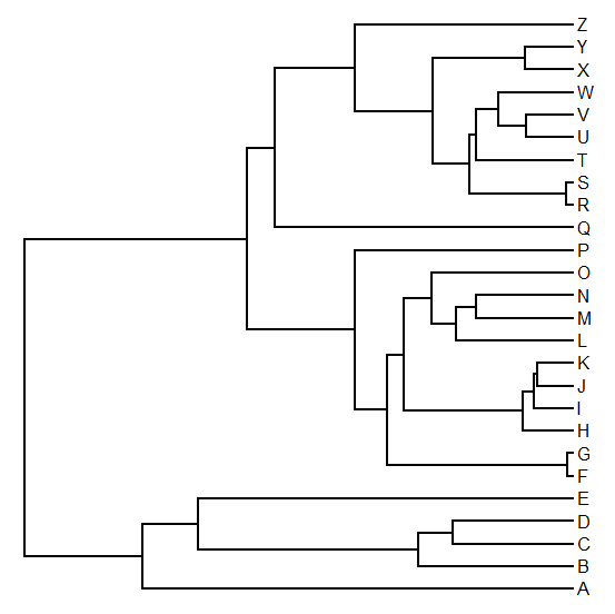
> plot(t1,edge.width=3,lend=2)
> title("read.tree")
> plot(t2,edge.width=3,lend=2)
> title("read.newick")
> bb<-"((((A),B),(C,D))),E);"
> t3<-read.tree(text=bb)
Error in if (sum(obj[[i]]$edge[, 1] == ROOT) == 1 && dim(obj[[i]]$edge)[1] > :
missing value where TRUE/FALSE needed
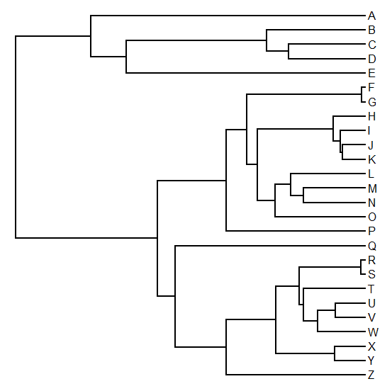
> t4<-read.newick(text=bb)
> layout(matrix(c(2,1),1,2))
> plot(t4,edge.width=3,lend=2)
Error in plot.phylo(t4, edge.width = 3, lend = 2) :
there are single (non-splitting) nodes in your tree; you may need to use collapse.singles()
> t4<-collapse.singles(t4)
> plot(t4,edge.width=3,lend=2)
> title("read.newick")

That's it.


Bug fix in brownieREML

$
0
0

A phytools user recently reported discrepant results between brownie.lite and brownieREML.** Both functions fit the multi-rate Brownian evolution model of O'Meara et al. (2006), the former using ML and the latter REML. To fit the model using REML we scale the branches & branch segments of the tree by the rate, and then we compute contrasts and maximize the probability of the contrasts given the rate parameters in our model.

(**Note that brownie.lite&brownieREML are not expected to give exactly the same results. REML should be unbiased, whereas ML is only asymptotically unbiased and will be slightly downwardly biased for small samples. That being said, the results should be quite similar for reasonable sample sizes in each rate regime.)

The bug is that the the order of the data in the input vector x need to be in the order of tree$tip.label, but this is not noted in the documentation and the function does not return an error if this is not the case. Oops.

OK, this has been fixed in the latest version of brownieREML. I have also improved the function code (which dates to the early days of phytools) so that it is a little cleaner.

This update, along with the totally new version of read.newick, are in a new non-CRAN build of phytools (phytools 0.2-84). Please keep the bug reports coming!

Common error in contMap

$
0
0

This is a commonly reported error from the function contMap:

contMap : Error in while (x > trans[i]) { : missed value TRUE / FALSE is required

I believe this is usually due to branches of zero length in the tree. For internal branches of zero length, this can be resolved using:

tree<-di2multi(tree)

Getting a list of all sets of tips separated by zero length (or a distance less than some arbitrary value)

$
0
0

An R-sig-phylo user asks:

Is there a way to detect and list all tips of a tree with 0 length in their terminal branches (essentially duplicated sequences)? Would also be great if it's possible to output them in groups so that it's clear which tips are identical to which.

I answered the first part as follows:

I would advise setting some "tolerance" value, below which you consider a terminal edge to be zero. Then try:

tol<-1e-8
x<-na.omit(tree$tip.label[tree$edge[tree$edge.length<= tol,2]])
attr(x,"class")<-NULL
attr(x,"na.action")<-NULL

This works great for the first part - the only problem is that it ignores the second part by not telling us what tips are separated by tol or less distance from which other tips.

Here is a solution that addresses that:

D<-cophenetic(tree)
tol<-1e-12 # say
x<-apply(D,1,function(x) names(which(x<=tol)))
x<-unique(x)
x<-x[sapply(x,length)>1]

Let's take the following tree:

and try it out:
> require(ape)
Loading required package: ape
> D<-cophenetic(tree)
> tol<-1e-12 # say
> x<-apply(D,1,function(x) names(which(x<=tol)))
> x<-unique(x)
> x<-x[sapply(x,length)>1]
> x
[[1]]
[1] "t9" "t11"

[[2]]
[1] "t10" "t12" "t13"

[[3]]
[1] "t3" "t14"

[[4]]
[1] "t6" "t17"

[[5]]
[1] "t1" "t18" "t19"

Cool - it works.

Function to collapse some subtrees into a star - while retaining the same total height of the tips

$
0
0

The following was recently requested via the R-sig-phylo mail list serve:

I'd like to collapse the descendants of a node, identified using something like node <- mrca(tree)["A", "B"]. I did not see a function in ape, geiger, phyloch, or picante to do something like collapse.descendants(node). Is there a package with a function like this?

This can be pretty easily done using the functions of phytools. Here's a little function to do this:

function(tree,node){
 tt<-splitTree(tree,split=list(node=node,bp=
  tree$edge.length[which(tree$edge[,2]==node)]))
 ss<-starTree(species=tt[[2]]$tip.label,branch.lengths=
  diag(vcv(tt[[2]])))
 ss$root.edge<-0
 tree<-paste.tree(tt[[1]],ss)
 return(tree)
}

And here is a quick demo:

> tree<-pbtree(n=50,scale=1)
> plotTree(tree,node.numbers=T,fsize=0.8)
> tree<-collapse.to.star(tree,fastMRCA(tree,"t7","t12"))
> tree<-collapse.to.star(tree,fastMRCA(tree,"t50","t18"))
> plotTree(tree,node.numbers=T,fsize=0.8)

Cool. That did exactly what we wanted tit to do. Note that every time we collapse a subtree, the node numbers of the tree will change - so we cannot use the node numbers from the original tree to collapse multiple subtrees (we need to recompute the target node each time).

New versions of phytools 3D methods

$
0
0

In my Evolution 2013 meeting talk (which I will put online soon), I showed a couple of old 3D visualization methods: a three-dimensional projection of the tree into morphospace ("phylomorphospace"); and a 3D traitgram visualization method in which x&y are phenotypic trait axes, while z represents the time since the root.

To make the plots I made a few minor updates to the two functions in which these methods are implemented: phylomorphospace3d and fancyTree(...,type="traitgram3d"). These updates are in a new phytools version (phytools 0.2-87). Here's a quick demo of how to create these as .gifs:

> require(phytools)
Loading required package: phytools
> packageVersion("phytools")
[1] ‘0.2.87’
> # simulate tree & data
> tree<-pbtree(n=40)
> X<-fastBM(tree,nsim=3)
> # create 3D phylomorphospace
> xx<-phylomorphospace3d(tree,X)
> movie3d(xx,duration=20,dir=".",movie= "phylomorphospace3d")
Will create: ./phylomorphospace3d.gif
Executing: convert -delay 1x10 phylomorphospace3d*.png phylomorphospace3d.gif
Deleting frames.
> # create 3D traitgram
> xx<-fancyTree(tree,type="traitgram3d",X=X[,1:2])
> movie3d(xx,duration=20,dir=".",movie="traitgram3d")
Will create: ./traitgram3d.gif
Executing: convert -delay 1x10 traitgram3d*.png traitgram3d.gif
Deleting frames.

That's it for now.

User control of node sizes in phylomorphospace

$
0
0

A phytools user requests:

Is there a way to turn off the internal nodes in the phylomorphospace function in phytools?

I decided to interpret this more generally as a request for user control over the size of the plotted points at terminal and internal nodes in a phylomorphospace (that is, a bivariate projection of the tree into morphospace) plot.

This was easy enough to add and is now an optional argument in the phylomorphospace function. Point size is controlled using the cex argument in points - which adjusts the plotted point size relative to the default (1.0). Code for the new version is here and I also posted a new phytools build (phytools 0.2-88) containing this update.

Here's a demo, using the original request above:

> require(phytools)
Loading required package: phytools
> packageVersion("phytools")
[1] ‘0.2.88’
> tree<-pbtree(n=30)
> X<-fastBM(tree,nsim=2)
> layout(matrix(c(1,2),1,2))
> plotTree(tree,mar=c(3.2,0.1,1.4,0.1))
> par(mar=c(4.1,4.1,2.1,0.5))
> phylomorphospace(tree,X,node.size=c(0,1.3),lwd=2, xlab="x",ylab="y",xlim=c(-4.2,2.2))
(Full resolution.)

Fix for bind.tip

$
0
0

At this year's Evolution meeting it was reported to me that bind.tip has some weird behavior if you try and attach a tip to the end of a terminal edge. One might want to do this if, say, identical haplotypes were removed for inference - and then one wanted to add them back in for plotting.

Here's a demo of the problem:

> tree<-pbtree(n=20)
> plotTree(tree,setEnv=TRUE,offset=0.7)
setEnv=TRUE is experimental. please be patient with bugs
> tiplabels()
> aa<-bind.tip(tree,"t21",where=1,position=0)
> plotTree(aa,setEnv=TRUE,offset=0.7)
setEnv=TRUE is experimental. please be patient with bugs
> tiplabels()

Holy cow! Weird, right? Instead of binding our new tip zero-length below the tip node, bind.tip is replacing the tip label of our target terminus! Note that this will not happen even if we add the the new tip just below the target tip.

In this case, bind.tip actually just wraps around the ape function bind.tree which attaches two trees together.

I have built a work-around into the latest version of bind.tip (source code now here). This is also in a new build of phytools (phytools 0.2-89). Let's verify that this works:

> require(phytools)
Loading required package: phytools
> packageVersion("phytools")
[1] ‘0.2.89’
> bb<-bind.tip(tree,"t21",where=1,position=0)
> plotTree(bb,setEnv=TRUE,offset=0.7)
setEnv=TRUE is experimental. please be patient with bugs
> tiplabels()
> bb$edge.length
[1] 0.49852021 0.90133001 0.63759396 0.36295139 0.00000000 0.00000000 ....

This fix is a bit of a hack - but at least it works.


phytools page temporarily down

$
0
0

The phytools page is temporarily down. This seems to be a server-wide issue and is thus not my fault - hopefully this will be fixed in the morning.

Upper triangle of a matrix to a vector by row

$
0
0

Say we want to get a square matrix into a vector. We can do:

to.upper<-function(X) X[upper.tri(X,diag=TRUE)]
but this will give us our upper triangular matrix as a vector by column, i.e.:
> X
       [,1]   [,2]   [,3]   [,4]   [,5]
[1,] -0.329 -0.825 -0.906  0.834  0.702
[2,]  1.195 -0.237 -1.132 -0.827  0.150
[3,] -0.097 -1.270 -1.397  0.450  0.791
[4,]  0.883 -0.574  1.538 -2.632  0.135
[5,]  1.993 -0.520 -0.071  0.094 -0.064
> to.upper(X)
[1] -0.329 -0.825 -0.237 -0.906 -1.132 -1.397  0.834 -0.827  0.450 -2.632  0.702  0.150  0.791  0.135 -0.064

If we want to get our upper triangular matrix as a vector by row (as I did), we can use:

to.upper<-function(X) t(X)[lower.tri(X,diag=TRUE)]
which works just as we'd hoped, i.e.:
> X
       [,1]   [,2]   [,3]   [,4]   [,5]
[1,] -0.329 -0.825 -0.906  0.834  0.702
[2,]  1.195 -0.237 -1.132 -0.827  0.150
[3,] -0.097 -1.270 -1.397  0.450  0.791
[4,]  0.883 -0.574  1.538 -2.632  0.135
[5,]  1.993 -0.520 -0.071  0.094 -0.064
> to.upper(X)
[1] -0.329 -0.825 -0.906  0.834  0.702 -0.237 -1.132 -0.827  0.150 -1.397  0.450  0.791 -2.632  0.135 -0.064

(Note that if we have a symmetric matrix than the upper triangular matrix by row & the lower triangular matrix by column are the same. Here I used a non-symmetric square matrix so that we could tell these apart.)

phytools page down again - new version of phytools submitted to CRAN

$
0
0

The phytools page is having problems again. This is a UMass-Boston server-wide issue, so there is not much I can do about it unfortunately (aside from complain to the system administrator). To make all the recent updates to the phytools package available to all users, however, I have just submitted a new version of phytools to CRAN. Hopefully this version is accepted and made available via the CRAN mirrors as well as in binary form soon.

Some updates in this version over the previous CRAN release (phytools 0.2-80) include the following:

1. A new function to add a legend to a plotted stochastic map tree (add.simmap.legend).

2. A new version of plotSimmap that sets the environmental variable "lastplot.phylo" to be compatible with ape functions nodelabels, tiplabels, and edgelabels.

3. A new version of findMRCA that can also (optionally) return the height above the root of the MRCA of a pair of taxa.

4. A robust Newick tree reader that can handle singleton nodes, if present.

5. A bug fix in brownieREML.

6. A new function (collapse.to.star) that collapses specified subtrees into a star tree, while retaining the same total height above the root for each tip.

7. New versions of the phytools 3D functions phylomorphospace3d and fancyTree(...,type="traitgram3d") that work a little better with the functions of rgl (described here).

8. User control of tip & internal node sizes in phylomorphospace..

9. A hacky work-around fix for the problem of attaching a new tip separated from an existing tip by zero lenth using bind.tip.

10. Finally, today, a fix to the broken function evol.vcv, which is the function implementing the method of Revell & Collar (2009).

Hopefully this new phytools update is accepted and posted to CRAN soon.

Static help pages for phytools

$
0
0

The html help pages in R are created dynamically from the .Rd manual pages; however it is also possible to create static .html help pages to post on the web (or have available for review without R open). I have done this now & posted them to the phytools page. For example, the static help page for make.simmap can be seen here. You can also see an index of all functions available in the latest version of phytools. Check it out.

For more information about building static html help pages in R, see the following link.

phytools page now hosted on 3rd party server

$
0
0

Happy 4th of July - the faculty pages web server at UMass-Boston has been suffering a lot of service interruptions over the past few days, so I have now moved the phytools page (http://www.phytools.org) to a new 3rd party provider. Hopefully that will take care of these service interruptions - and, of course, phytools is always available through CRAN.

Correction: the link above to http://www.phytools.org originally pointed to the wrong web address. Fixed.

Plotting 'partial' circular trees

$
0
0

At this year's Evolution meeting in Snowbird, Utah, I saw a very nice poster by Patrick Fuller of the Wainwright Lab at UCDavis. One cool attribute of the poster was that he had a half circular phylogeny aligned to the bottom of this poster. My immediate thought, naturally, was that phytools should do this.

I have now added this capability to the functions plotSimmap (as well as plotTree, which uses plotSimmap internally). I have included these updates in a new non-CRAN release of phytools (phytools 0.2-91), which can be downloaded and installed from source.

Doing this was not hard. Basically, when we are deciding the circular positions of all the terminal edges of the tree, we start by ordering them cladewise, and then we evenly space the tips from 0 through 2π before wrapping them into our circular space. (I describe this a little more here.) To plot a partial fan tree, we just decide what fraction, θ, of the circle we want to use, then we space our terminal edges, instead of evenly from 0 to 2π, evenly from 0 through 2πθ. Aside from resizing our plot axes to match - that's pretty much all there is to it.

Here's a quick demo of the results:

> library(phytools)
> packageVersion("phytools")
[1] ‘0.2.91’
> data(anoletree)
> plotSimmap(anoletree,type="fan",part=0.5,fsize=0.9, ftype="i")
no colors provided. using the following legend:
    CG     GB      Non-     TC     TG        Tr        TW
"black"  "red"  "green3" "blue" "cyan" "magenta"  "yellow"

Note: type="fan" is in development.
Many options of type="phylogram" are not yet available.

> ss<-sort(unique(getStates(anoletree,"tips")))
> add.simmap.legend(colors=setNames(palette()[1:length(ss)],ss))
Click where you want to draw the legend
(Click here for full resolution.)

Pretty cool. That's about what we were going for. Here's a smaller, simulated 1/4 fan tree - again, with a mapped discrete character:

> Q<-matrix(c(-1,1,1,-1),2,2)
> tree<-sim.history(pbtree(n=40,scale=1),Q,anc=1)
> plotSimmap(tree,colors=setNames(c("blue","red"),1:2), type="fan",part=0.25,lwd=4)

Note: type="fan" is in development.
Many options of type="phylogram" are not yet available.

> add.simmap.legend(colors=setNames(c("blue","red"),1:2))
Click where you want to draw the legend

That's it.

New version of plotBranchbyTrait with full user control of plotting options

$
0
0

Today I received the following request from a colleague regarding the phytools function plotBranchbyTrait:

A PhD student of mine is trying to use your function plotBranchbyTrait to plot a phylogeny where the branch colors reflect the rate of molecular evolution .... He has managed to plot the tree with the branch colors and that part works very nicely, but when trying to offset the tip labels (species names) or modifying the edge.width he gets a message saying that the argument "label.offset" (or "edge.width") is matched by multiple actual arguments.... Can you assist us as why you think we're getting these messages? Any tricks to offset the species names?

plotBranchbyTrait differs from other similar functions in phytools (such as densityMap and contMap) in that it requires a single input value for the mapped trait per edge, and then plots that trait value on a color gradient scale - but uniformly for each branch.

The truth is, I developed this function primarily to help a colleague - so it is not endowed with the full range of plotting options. Unlike the vast majority of tree plotting functions in phytools, this one calls plot.phylo from the ape package internally - rather than plotSimmap in phytools.

This afternoon, I took a the twenty minutes (or so) required to pass control of all* (*with the exception of a couple, such as edge.color, which don't make sense) to the user. In so doing, I've kept the non-optional arguments of plotBranchbyTrait the same, although I've changed a few of the internal defaults - just to make for nicer plots. (For instance, I discovered that the default x & y limits meant that the legend was being plotting out of bounds in many instances.)

The updated code for plotBranchbyTrait is here, but I have also posted a new version of phytools (phytools 0.2-93), which can be downloaded and installed from source. (For more information on installing packages from source, search the web.)

Here's the usual demo:

> library(phytools)
> packageVersion("phytools")
[1] ‘0.2.93’
> tree<-pbtree(n=50)
> x<-fastBM(tree)
> plotBranchbyTrait(tree,x,mode="tips",edge.width=4, prompt=TRUE)
Click where you want to draw the bar

For fun, we can compare to contMap, which interpolates smoothly along each internal & terminal edge. (Of course, plotBranchbyTrait can also be used for any arbitrary trait in which we have a state on a continuous scale at each edge of the tree.) These two plots should look very similar - it is just a matter of whether or not our eyes can easily distinguish between continuously & abruptly changing colors.

> XX<-contMap(tree,x,lims=c(-3.5,1.5))
> XX$cols[]<-rainbow(1001,start=0.7,end=0)
> plot(XX,outline=F,lwd=4,legend=0.82)

Virtually the same to my eye!


Phylomorphospace with time since the root projected using a color gradient

$
0
0

Two different people (Marcio Pie and a student whose name has somehow slipped my mind - please identify yourself!) independently suggested to me recently that I could use a similar approach to that employed when overlaying a posterior density map from stochastic mapping on a phylomorphospace to project time since the root of the tree onto a phylomorphospace. In theory, this would help overcome the difficulty that all temporal information about the phylogeny is lost when it is projected into morphospace.

Well, this is quite easy** (**that is, easy only because I've already programmed all the pieces in phytools) to do. Here's a hack using simulated data.

First let's load phytools & simulate tree & data:

> require(phytools)
Loading required package: phytools
> packageVersion("phytools")
[1] ‘0.2.93’
> # simulate tree & data
> tree<-pbtree(n=30,scale=100)
> X<-fastBM(tree,nsim=2)
Next, we're going to create an object of class "contMap". This is just a placeholder into which we'll slot our temporal data:
# unfortunately, there's no way to prevent this from plotting
AA<-contMap(tree,X[,1])
Now, we'll swap our color palette (although we don't need to - this is just an arbitrary decision); and then we'll substitute information about the height from the root for our trait data mapped onto the tree:
> AA$cols[]<-rainbow(1001,start=0.7,end=0)
> H<-nodeHeights(tree)
> h<-max(H)
> for(i in 1:nrow(H)) names(AA$tree$maps[[i]])<- round((H[i,1]+cumsum(AA$tree$maps[[i]]))/h*1000)
> # check to verify that temporal information is correct
> plot(AA,legend=FALSE)
Finally, let's plot our phylomorphospace with color as a temporal axis:
> phylomorphospace(AA$tree,X,colors=AA$cols,lwd=3, node.by.map=TRUE,xlab="trait 1",ylab="trait 2")
> add.color.bar(2,AA$cols,title="time from the root", lims=c(0,h),digits=1)
Click where you want to draw the bar
(Click here for full size.)

The final step (add.color.bar(...)) is the biggest hack of all as it only works because I artfully positioned it close enough to the x axis so that the bottom legend text is hidden!

Try it out!

Adding a scale bar to a partial circular tree

$
0
0

Here's a neat trick that I thought of yesterday. We can pretty easily add a scale bar to a partial circular tree created using plotTree(...,type="fan") in the phytools package, and here's how:

> library(phytools)
> packageVersion("phytools")
[1] ‘0.2.93’
> # for this demo - simulate a tree of length 100
> tree<-pbtree(n=100,scale=100)
> # plot it
> # (you'll probably need to tweak 'part' to fit the axis)
> plotTree(tree,type="fan",part=0.93,fsize=0.9)

Note: type="fan" is in development.
Many options of type="phylogram" are not yet available.

> # ok, now plot the axis
> h<-max(nodeHeights(tree))
> axis(1,pos=-0.05*h,at=seq(0,h,by=h/2),lwd=2)
> text(x=0.5*h,y=-0.25*h,"time")

That's pretty cool.

Rotating all the nodes in a tree (or a set of nodes)

$
0
0

I just wrote a utility function that wraps around rotate in the ape package to rotate a set of nodes in a tree (including nodes="all"). It also addresses this weird problem that I discovered that results when a bunch of rotations are applied to a tree the "phylo" can become non-compliant with certain ape & phytools functions because the order of the tip numbers in tree$edge is not 1:n for n tips.

Here's the function:

rotateNodes<-function(tree,nodes,polytom=c(1,2),...){
  n<-length(tree$tip.label)
  if(nodes[1]=="all") nodes<-1:tree$Nnode+n
  for(i in 1:length(nodes))
    tree<-rotate(tree,nodes[i],polytom)
  if(hasArg(reversible)) reversible<-list(...)$reversible
  else reversible<-TRUE
  if(reversible){
    ii<-which(tree$edge[,2]<=n)
    jj<-tree$edge[ii,2]
    tree$edge[ii,2]<-1:n
    tree$tip.label<-tree$tip.label[jj]
  }
  return(tree)
}

Let's try it:

> tree<-pbtree(n=26)
> tree$tip.label<-LETTERS
> plotTree(tree)
> tree<-rotateNodes(tree,"all")
> plotTree(tree)

Small update to contMap and densityMap to suppress plotting

$
0
0

The phytools functions densityMap and contMap invisibly return objects of class "densityMap" and "contMap", respectively. However there was previously no way to suppress plotting - which might be desired if (say) the density map was being produced to project onto a phylomorphospace plot. Today I added the capacity to turn off plotting to both functions and they are included in the latest phytools build (phytools 0.2-05).

Here's a demo, using simulated data &densityMap:

> # load phytools
> require(phytools)
Loading required package: phytools
> packageVersion("phytools")
[1] ‘0.2.95’
> # simulate data for a discrete character
> Q<-matrix(c(-1,1,1,-1),2,2)
> rownames(Q)<-colnames(Q)<-0:1
> tree<-sim.history(pbtree(n=40,scale=1),Q)
> # simulate data for two continuous characters
> # with a rate matrix that varies by state
> R<-setNames(list(matrix(c(1,0,0,1),2,2),
  matrix(c(5,4,4,5),2,2)),0:1)
> X<-sim.corrs(tree,R)
> # conduct stochastic map
> trees<-make.simmap(tree,tree$states,nsim=100)
make.simmap is sampling character histories conditioned on the transition matrix
Q =
           0          1
0 -0.7416182  0.7416182
1  0.7416182 -0.7416182
(estimated using likelihood);
and (mean) root node prior probabilities
pi =
  0  1
0.5 0.5
Done.
> # create a density map but suppress plot
> XX<-densityMap(trees,plot=FALSE)
sorry - this might take a while; please be patient
> # project density map onto phylomorphospace
> par(mar=c(5.1,4.1,2.1,2.1))
> phylomorphospace(XX$tree,X,colors=XX$cols, node.by.map=TRUE,lwd=3,xlab="trait 1",ylab="trait 2")
(Click here for full size.)

Visualizing multivariate comparative data on trees: multipanel phylomorphospace plotting

$
0
0

This is kind of cool: a multipanel phylomorphospace plot for four different traits with a set of contMap univariate plots on the diagonal:

(Click here for higher resolution.)

Here's how I did it (ignoring the data simulation). Note that a new, non-CRAN version of phytools (phytools 0.2-96) is required to do this.

m<-ncol(X)
par(mfrow=c(m,m))
par(cex=0.6)
par(mar=c(0,0,0,0))
par(oma=c(5,5,3,3))
m<-ncol(X)
for(i in 1:m) for(j in 1:m){
  if(i==j) contMap(tree,X[,i],legend=FALSE,lwd=2,outline=F,
    fsize=0.5)
  else {
    phylomorphospace(tree,X[,c(j,i)],lwd=1,
      node.by.map=TRUE,axes=FALSE)
    if(i==1) axis(side=3) # top row
    if(i==m) axis(side=1) # first column
    if(j==1) axis(side=2) # bottom row
    if(j==m) axis(side=4) # last column
  }
}
par(cex=0.9)
mapply(title,xlab=colnames(X),adj=
  seq(0,(m-1)/m,1/m)+1/(2*m),MoreArgs=
  list(outer=TRUE,cex=0.9))
mapply(title,ylab=colnames(X)[m:1],adj=
  seq(0,(m-1)/m,1/m)+1/(2*m),MoreArgs=
  list(outer=TRUE,cex=0.9))
Viewing all 800 articles
Browse latest View live