Quantcast
Viewing all 802 articles
Browse latest View live

New version of fastAnc; new build of phytools

I just posted a new version of the function fastAnc for (relatively) fast ancestral character estimation. The function is previously described here. The main addition to this new version is that now the function (optionally) computes the variance on the ancestral state estimates based on equation (6) of Rohlf (2001), as well as (optionally) 95% confidence intervals on the states. The updated code is here; however, I have also posted a new build of phytools - which can be downloaded here and installed from source.

Note that equation (6) of Rohlf (2001) only gives the relative variance on the ancestral state estimate at the root node. To scale that estimate to our data, we need to multiply by the phylogenetic variance for our continuous trait. This can be computed as the mean square of the contrasts. Once we have the variances, we can compute our 95% CIs on the estimates as the estimates +/- 1.96 × the square root of the variances.

I didn't realize this when I was writing the function, but it turns out to be the case that this update to fastAnc depends on ape>= 3.0-7 (i.e., the newest version of ape as of the date of writing). This is because the options in the ape function for independent contrasts, pic, were expanded in the latest release to include the option of returning the tree with branches scaled to expected variance - which we can conveniently exploit to do the calculation of equation (6) in Rohlf.

I should also point out that the 95% CIs obtained by this function differ in a substantial way from the 95% CIs computed in ace. Specifically, the 95% CIs computed in ace would seem to be too small. We can show this relatively easily by simulation, as follows:

> onCI.ace<-onCI.fastAnc<-vector()
> N<-100
> for(i in 1:1000){
+ tree<-pbtree(n=N)
+ x<-fastBM(tree,internal=TRUE)
+ a<-fastAnc(tree,x[1:N],vars=TRUE,CI=TRUE)
+ onCI.fastAnc[i]<-sum((x[1:tree$Nnode+N]>a$CI95[,1])*(x[1:tree$Nnode+N]< a$CI95[,2]))/tree$Nnode
+ b<-ace(x[1:N],tree,CI=TRUE)
+ onCI.ace[i]<-sum((x[1:tree$Nnode+N]>b$CI95[,1])*(x[1:tree$Nnode+N]< b$CI95[,2]))/tree$Nnode
+ }
There were 24 warnings (use warnings() to see them)
> warnings()
Warning messages:
1: In sqrt(diag(solve(h))) : NaNs produced
2: In sqrt(diag(solve(h))) : NaNs produced
3: ...
> # this should be 0.95
> mean(onCI.fastAnc)
[1] 0.9483737
> mean(onCI.ace,na.rm=TRUE)
[1] 0.6738759

This simulation shows that although our 95% CIs computed in fastAnc include the generating values almost exactly 95% of the time (94.8% across 1000 simulations with 99 estimated ancestral states per simulation), ace CIs only include the generating value about 67% of the time.

I'm not exactly sure why this is the case, but my best guess is based on the warnings which tell us that the Hessian is being used to compute the standard errors of the parameter estimates and thus the CIs. This is an asymptotic property of the likelihood surface, and for finite sample this approximation can be quite bad (as we see above).

Function to get the sister(s) of a node or tip

I just posted a new utility function, getSisters, that takes as input a tree and a node or tip number or label, and returns the sister node or tip numbers or labels. It has two modes: mode="number", which returns node or tip numbers as an integer or vector; and mode="label" which returns a list with up to two components - one component for node labels (if available) or numbers, and the other component with tip labels.

The code for the function is here, but it also in the most recent build of phytools: phytools 0.2-18.

Here's a quick demo:
> require(phytools)
> tree<-rtree(n=12)
> plotTree(tree,node.numbers=TRUE)
Image may be NSFW.
Clik here to view.
> getSisters(tree,19)
[1] 23
> getSisters(tree,18,mode="label")
$tips
[1] "t10"

You get the idea. We can also collapse some branches so that some tips or nodes have multiple sister tips or nodes:
> tree$edge.length[which(tree$edge[,2]==18)]<-0
> tree$edge.length[which(tree$edge[,2]==23)]<-0
> tree$edge.length[which(tree$edge[,2]==20)]<-0
> tree$edge.length[which(tree$edge[,2]==21)]<-0
> tree<-di2multi(tree)
> plotTree(tree,node.numbers=T)
Image may be NSFW.
Clik here to view.
> getSisters(tree,18,mode="label")
$tips
[1] "t8" "t2" "t10"

> getSisters(tree,"t4",mode="label")
$nodes
[1] 19

$tips
[1] "t3" "t11"

That's it.

New version of phytools on CRAN (phytools 0.2-20)

A new version of phytools (phytools 0.2-20) is now on CRAN. Presently you can download the source code for this version from the phytools homepage or phytools CRAN page and install from source. Windows and Mac OS binaries should be built soon and eventually these will percolate through all the different CRAN mirrors.

Due to updates in a couple of different functions, phytools now depends on ape ≥ 3.0-7 (the latest version of ape as of the present date) and imports from phangorn ≥ 1.6-3.

Here's a brief list of some of the updates in phytools 0.2-20 relative to the last CRAN version (0.2-1):

1. A new function, splitplotTree, to plot a phylogeny in multiple columns or plotting windows.

2. A new function, bind.tip, for adding a single tip to the tree (1, 2).

3. A couple of critical bug fixes for phyl.RMA (1, 2).

4. A significant update to the function matchNodes which matches nodes between trees based either on the descendant tips from each node or on the distances from nodes to the tips in the tree.

5. A new utility function, applyBranchLengths, which applies the branch lengths from one tree to other topologically identical phylogenies.

6. New versions of ancThresh (e.g., here) and user control of phytools function plotThresh and threshDIC.

7. A new function, add.random, to add tips at random to a phylogeny.

8. An important update to pgls.Ives, to accept individual data, rather than just species means and standard errors.

9. A new function, orderMappedEdge, to reorder the "phylo" object mapped.edge in SIMMAP style trees.

10. A new version of the function, mrp.supertree, for MRP supertree estimation (1, 2).

11. Update to the function phylANOVA for phylogenetic ANOVA based on Garland et al. (1993).

12. A new version of fastAnc to compute the variances and 95% CIs on ancestral states.

13. A new function, getSisters, to get the node(s) or tip(s) that are sister to a focal node.

14. Minor updates to several functions including add.everywhere, allFurcTrees, anc.Bayes, anc.ML, anc.trend, ancThresh, brownie.lite, estDiversity, evol.rate.mcmc, evol.vcv, evolvcv.lite, exhaustiveMP, fancyTree, fitBayes, make.simmap, optim.phylo.ls, phyl.pairedttest, phylomorphospace, plotSimmap, reroot, sim.corrs, sim.history, sim.rates, and write.simmap.

15. Finally, as I mentioned before, a change in the dependency relationship with ape and phangorn. phytools now depends on ape ≥ 3.0-7 - but imports from phangorn (≥ 1.6-3).

Visualizing uncertainty in a 'traitgram'

For a variety of a reasons, I've been thinking about clever ways to try and visualize uncertainty in ancestral state estimates. Here is one attempt using an adaptation of the phytools function phenogram. This function plots a projection of the tree into a two dimensional space defined by time since the root (on the x) and phenotype. Note that to run this I had to first add the optional argument add to phenogram, so you will need to download and load the source (phenogram.R) to get this to work.

library(phytools)
# load source
source("phenogram.R")
# simulate tree & data
tree<-pbtree(n=20)
plotTree(tree)
x<-fastBM(tree)
# estimate ancestors
A<-fastAnc(tree,x,CI=TRUE)
tree<-paintSubTree(tree,node=length(tree$tip)+1,"1")
# our transparencies
trans<-as.character(floor(0:50/2))
trans[as.numeric(trans)<10]<-
  paste("0", trans[as.numeric(trans)<10],sep="")
# plot
for(i in 0:50){
  p<-i/length(trans)
  phenogram(tree,c(x,(1-p)*A$CI95[,1]+p*A$ace), colors=setNames(paste("#0000ff",trans[i+1],sep=""),1), add=i>0)
  phenogram(tree,c(x,(1-p)*A$CI95[,2]+p*A$ace), colors=setNames(paste("#0000ff",trans[i+1],sep=""),1), add=TRUE)
}
phenogram(tree,c(x,A$ace),add=TRUE, colors=setNames("white",1))
One word of caution about this visualization. Since I plot uncertainty using transparent colors, it can be difficult to impossible to extract uncertainty about any specific ancestral node from this plot. However what the plot is good at showing is the probability density of all hypothetical ancestors at any time slice through the tree.

Type I error and power of the 'phylogenetic ANOVA'

There are a couple of different statistical methods that are commonly referred to as the phylogenetic ANOVA.

The phylogenetic ANOVA is generally meant to refer to the simulation approach of Garland et al. (1993). Under this method, we fit the ANOVA model in the typical way - but then we conduct Brownian numerical simulations on the tree to obtain a null distribution of the model test statistic (F). This Monte Carlo simulated null distribution is used for hypothesis testing. The Garland et al. (1993) phylogenetic ANOVA is implemented in the function phy.anova from the geiger package, as well as in the phytools function phylANOVA, which adds post-hoc tests.

The second approach is what I'm going to refer to as the phylogenetic generalized least squares (GLS) ANOVA. Under this model we used the mechanics of GLS to fit a linear model in which the residual error of the model has phylogenetic autocorrelation. This is analogous, and mathematically equivalent, to fitting a phylogenetic regression (sensu Grafen 1989), as described in Rohlf (2001).

The disadvantage of the former approach is that it cannot be used to estimate the coefficients of the fitted ANOVA model - only the p-value of this fit. This is because the OLS estimators (although statistically unbiased) are not minimum variance - and may have very high variance (probably depending on the phylogenetic structure of the independent variable). By contrast, GLS has the advantage of giving unbiased and minimum variance estimators of the fitted model coefficients - that is, conditioned on our model for the residual error being correct.

In spite of the similarity of the goals of these two different approaches, to my knowledge no prior study has compared their type I error or power. The code below can be used to estimate the type I error of each approach, as well as standard OLS (i.e., ignoring the phylogeny):

# load required packages
require(phytools)
require(nlme)

# number of replicates
N<-200

# balanced tree
tree<-compute.brlen(stree(n=128,type="balanced"))

# transition matrix for simulation
Q<-matrix(c(-2,1,1,1,-2,1,1,1,-2),3,3)
rownames(Q)<-colnames(Q)<-c(0,1,2)

# simulate discrete character
mtrees<-replicate(N,sim.history(tree,Q),simplify=FALSE)
class(mtrees)<-"multiPhylo"

# plot (just for fun)
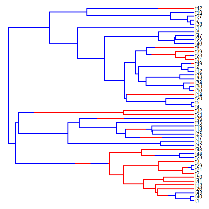
cols<-c("white","blue","red"); names(cols)<-0:2
foo<-function(x){
  plotTree(x,ftype="off",lwd=5)
  plotSimmap(x,cols,pts=FALSE,ftype="off",lwd=3,add=TRUE)
}
lapply(mtrees,foo)

# conduct simulations under the null
anovaOLS<-anovaPGLS<-anovaGarland<-list()
for(i in 1:N){
  b<-c(0,0,0)
  x1<-factor(mtrees[[i]]$states,levels=c(0,1,2))
  e<-fastBM(mtrees[[i]])
  y<-as.vector(b%*%t(model.matrix(~0+x1))+e)
  anovaOLS[[i]]<-anova(gls(y~x1,data.frame(y,x1)))
  anovaPGLS[[i]]<-anova(gls(y~x1,data.frame(y,x1), correlation=corBrownian(1,mtrees[[i]])))
  anovaGarland[[i]]<-phylANOVA(mtrees[[i]],x1,y,posthoc=F)
  print(paste("replicate",i))
}

# extract the p-values of the fitted models
pOLS<-sapply(anovaOLS,function(x) x$'p-value'[2])
pGLS<-sapply(anovaPGLS,function(x) x$'p-value'[2])
pGarland<-sapply(anovaGarland,function(x) x$Pf)

From here it is simple to get the type I error rate for each method:
> # get type I error
> typeI.OLS<-mean(pOLS<=0.05)
> typeI.GLS<-mean(pGLS<=0.05)
> typeI.Garland<-mean(pGarland<=0.05)
> typeI.OLS
[1] 0.85
> typeI.GLS
[1] 0.04
> typeI.Garland
[1] 0.06

So, it looks like Garland et al.'s simulation method and phylogenetic GLS both have appropriate type I error rates when there is no effect of the independent variable - but ignoring the phylogeny entirely can result in very high type I error. I should note that the simulation approach - using phylogenetic simulation of x and Grafen's branch lengths - is kind of the "worst case scenario" for ignoring phylogeny.

We can loop around this code and ask whether the power to detect an effect of various sizes differs between PGLS-ANOVA and Garland et al.'s simulation approach. Here is the code I used as well as the result. To be able to run through this a little quicker, I decided to use only the first 100 trees from my prior simulation.

# power analysis
N<-100
power.GLS<-typeI.GLS; power.Garland<-typeI.Garland
anovaPGLS<-anovaGarland<-list()
for(i in 1:10){
  for(j in 1:N){
    # simulate an effect
    # note that this relative to a variance between tips
    # separated by the root of 1.0
    b<-c(0,-0.1*i,0.1*i)
    x1<-factor(mtrees[[j]]$states,levels=c(0,1,2))
    e<-fastBM(mtrees[[j]])
    y<-as.vector(b%*%t(model.matrix(~0+x1))+e)
    anovaPGLS[[j]]<-anova(gls(y~x1,data.frame(y,x1), correlation=corBrownian(1,mtrees[[j]])))
    anovaGarland[[j]]<-phylANOVA(mtrees[[j]],x1,y, posthoc=F)
    print(paste("effect",i*0.1,"- replicate",j))
  }
  # extract the p-values of the fitted models
  pGLS<-sapply(anovaPGLS,function(x) x$'p-value'[2])
  pGarland<-sapply(anovaGarland,function(x) x$Pf)
  # get power
  power.GLS[i+1]<-mean(pGLS<=0.05)
  power.Garland[i+1]<-mean(pGarland<=0.05)
}
plot(0:10/10,power.GLS,type="b",ylim=c(0,1), xlab="effect size",ylab="power")
lines(0:10/10,power.Garland,type="b")
lines(c(0,1),c(0.05,0.05),lty=2)
text(x=1,y=0.95,"PGLS",pos=2,offset=0)
text(x=1,y=0.7,"Garland et al.",pos=2,offset=0)
So, there you have it. If I've done this properly, it suggests that the Garland et al. simulation method has the correct type I error - but relatively low power compared to PGLS. Cool.

One caveat that I'd like to attach to all of this is that I've always found the presumed generating process - one in which the mean structure effectively evolves 'saltationally' (changing state spontaneously whenever the discrete character changes state) but the error structure evolves by Brownian evolution - to feel more than a little artificial.

That being said, I still feel that this result might interest some people. Could this be a published 'note?' I'm not sure, but feedback is welcome.

'Tangled trees' from add.random

Today I received the following bug report about the relatively new phytools function add.random:

I had a question about the add.random function you posted on your phytools blog a few weeks ago. Occasionally when I add a set of tips, the resulting phylogeny plots so that some branches cross. Anecdotally, it seems to happen only (or at least more often) when the number of added tips > number of ‘real’ tips in the tree (but I haven’t looked at this much). The phylo.object seems to function as I’d expect otherwise so it seems to just be a plotting thing, but I don’t know enough about how plot.phylo reads the phylo object to know for sure.

Indeed this bug is quite easy to replicate:
> set.seed(6)
> tree<-pbtree(n=5)
> treeAdded<-add.random(tree,n=10)
> layout(c(1,2))
> plotTree(tree); plotTree(treeAdded)

Obviously, there is branch crossing here. I'm going to pass the buck a bit here and mention that althoughadd.random calls the phytools function bind.tip (1,2) internally, bind.tip is little more than a thinly coded wrapper for the 'ape' function bind.tree.

Branch crossing appears to occasionally occur because both plot.phylo (in ape) and plotTree (in phytools) assume a particular ordering for the edges and tips in tree$edge, which sometimes fails to be satisfied when a lot of tips have been added to the tree. Luckily, this only affects plotting (so far as I know), and none of the other functions of the "phylo" object.

Fortunately, this is also incredibly easy to solve. The following are two different functions that will "untangle" the tree, so to speak:

untangle1<-function(x) reorder(reorder(x,"pruningwise"))
## or
untangle2<-function(x) read.tree(text=write.tree(x))

We can try it out on our previous example, from above:
> treeUntangled1<-untangle1(treeAdded)
> treeUntangled2<-untangle2(treeAdded)
> layout(c(1,2,3))
> plotTree(treeAdded)
> plotTree(treeUntangled1)
> plotTree(treeUntangled2)

Since both functions do the job, we can also ask if one is more computationally efficient than the other. Let's do this using a much bigger tree. We'll do that using system.time:
> tree<-pbtree(n=5)
> # this takes a while!
> tree<-add.random(tree,n=2000)
> plotTree(tree,ftype="off",lwd=1)
> # lots of tangles!
> system.time(tree1<-untangle1(tree))
  user  system elapsed
     0       0       0
> system.time(tree2<-untangle2(tree))
  user  system elapsed
  0.37    0.00    0.37
> plotTree(tree1,ftype="off",lwd=1)
> # untangled! (tree2 is the same)
> all.equal(tree,tree1)
[1] TRUE
> all.equal(tree,tree2)
[1] TRUE

It's a small difference, but the reorder.phylo method is lightning fast! One important note - users should be aware that the tip & node numbers of our tree change when we untangle it.

That's it. I will write a new utility function, untangle, that will do this and also untangle SIMMAP style "phylo" objects. When I get around to that, I'll post it.

More on 'untangling' misplotted trees

I just posted a new function, untangle, which attempts to "untangle" branch crossing resulting from bind.tree or other functions.

It has two different methods: method="reorder" and method="read.tree" (as described here), and will also attempt to untangle SIMMAP style trees automatically using reorderSimmap. I've included it in a non-CRAN version of phytools (phytools 0.2-21), which can be downloaded from the phytools website and installed from source. This version also includes an updated version of phenogram.

Here's a quick demo of untangle with SIMMAP style trees:
> install.packages("phytools_0.2-21.tar.gz",type="source", repos=NULL)
...
* DONE (phytools)
> require(phytools)
Loading required package: phytools
> tree<-add.random(pbtree(n=5),n=45)
> Q<-matrix(c(-1,1,1,-1),2,2)
> rownames(Q)<-colnames(Q)<-c(1,2)
> cols<-setNames(c("blue","red"),c(1,2))
> mtree<-sim.history(tree,Q,anc="1")
> plotSimmap(mtree,cols,pts=F,lwd=3)
> mtree<-untangle(mtree)
> plotSimmap(mtree,cols,pts=F,lwd=3)

That's it.

New version of package for numerical analyses in evolutionary biology

I just added a new function to my little R package 'popgen' for numerical analyses and simulation in evolution and population genetics (see my previous post on this here). The function is called hawk.dove and does numerical analysis of a simple discrete-time hawk-dove model. It then shows the result in a two panel plot. The first panel gives the frequencies of each phenotype through time; whereas the second plot gives the mean fitness of the population and the mean fitness of each strategy. The idea is to play with the payoff matrix to see how the behavior of the model changes. Coexistence of both hawk and dove strategies, or extinction of one or the other, are all possible.

Here's a demo. First download the package source (popgen 0.2).

> install.packages("popgen_0.2.tar.gz",type="source", repos=NULL)
...
* DONE (popgen)
> payoff<-matrix(c(0.6,1.5,0.5,1.0),2,2,byrow=T)
> colnames(payoff)<-rownames(payoff)<-c("hawk","dove")
> payoff
    hawk dove
hawk  0.6  1.5
dove  0.5  1.0
> hawk.dove(M=payoff,time=50)
Pay-off matrix:
    hawk dove
hawk  0.6  1.5
dove  0.5  1.0

That's it.

On the shape of trees with random taxa addition or subtraction

Since I have a new function for add tips at random to a tree; and it is even easier to write a function to drop tips randomly from the tree - i.e., here it is:
drop.random<-function(tree,n=1)
   tree<-drop.tip(tree,tip=sample(tree$tip.label)[1:n])
I thought it might be fun to look at the effects of adding or subtracting tips at random from the tree. We already know that random missing taxa tends to create trees with longer than expected terminal edges - seemingly a slow-down in the rate of lineage diversification through time.

This is not very scientific, but first let's look at the LTT and Pybus & Harvey's (2000) γ for a single tree that we initiate with 100 species and then add to randomly using add.random in increments of 10. Here's our code (minus creating the video):
require(phytools)
tree<-pbtree(n=100,scale=1)
mas<-900
for(i in 1:(mas/10+1)){
  x<-ltt(tree,plot=FALSE)
  plot(x$times[2:length(x$times)],x$ltt[2:length(x$ltt)], xlab="time",ylab="lineages",log="y",type="l",xlim=c(0,1), ylim=c(2,max(x$ltt)))
  lines(c(0,1),c(2,max(x$ltt)),lty=2)
  text(x=0,y=max(x$ltt),paste("N = ",length(tree$tip), "\n","gamma = ",round(x$gamma,3),sep=""),adj=c(0,1))
  tree<-add.random(tree,n=10)
}

And here's the result:

OK, next, let's do the opposite - start with 1000 taxa and drop taxa random. First the code:
drop.random<-function(tree,n=1)    tree<-drop.tip(tree,tip=sample(tree$tip.label)[1:n])
require(phytools)
tree<-pbtree(n=1000,scale=1)
menos<-900
for(i in 1:(menos/10+1)){
x<-ltt(tree,plot=FALSE)
  plot(x$times[2:length(x$times)],x$ltt[2:length(x$ltt)],xlab="time", ylab="lineages",log="y",type="l",xlim=c(0,1), ylim=c(2,max(x$ltt)))
  lines(c(0,1),c(2,max(x$ltt)),lty=2)
  text(x=0,y=max(x$ltt),paste("N = ",length(tree$tip), "\n","gamma = ",round(x$gamma,3),sep=""),adj=c(0,1))
  tree<-drop.random(tree,n=10)
}

And the video:

Adding taxa at random, at least by our algorithm, does not seem to affect tree shape all that much; but subtracting random tips, as we expected, makes γ turn progressively more and more negative.

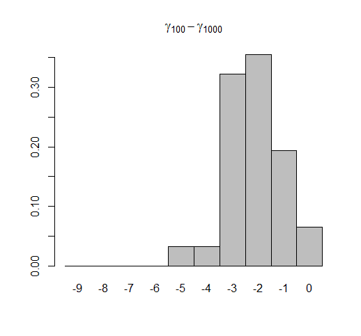
To see if this is idiosyncratic to the specific trees we started with, why don't we replicate the entire process (i.e., 900% addition or subtraction) in a single step for, say, 30 random pure-birth trees. Here's what that looks like. First, adding tips randomly:
XX<-matrix(NA,31,2,dimnames=list(NULL,c("gamma100","gamma1000")))
require(phytools)
for(i in 1:31){
  tree<-pbtree(n=100)
  XX[i,1]<-ltt(tree,plot=F)$gamma
  tree<-add.random(tree,900)
  XX[i,2]<-ltt(tree,plot=F)$gamma
}
colMeans(XX)
ZZ<-hist(XX[,2]-XX[,1],plot=F,breaks=-9.5:0.5)
barplot(ZZ$density,names=ZZ$mids,space=0,main=expression(gamma[100]-gamma[1000]))

And the results:
> colMeans(XX)
 gamma100  gamma1000
0.3568899 -1.9163830
And if we do the same thing dropping tips, here are the results:
> colMeans(YY)
 gamma100  gamma1000
-6.1072618 0.2275565
So, on the face of it, it seems as though adding taxa randomly (from 100 to 1000 species in the tree) or dropping taxa (from 1000 to 100) both result in a decrease in γ - however the scale of decrease is highly asymmetrical, with random subtraction resulting in a much greater decrease in γ.

At the start of this little experiment I wasn't sure if random addition of taxa would increase or decrease γ, and in the end it seems to decreaseγ but sometimes only a little.

New function to write trees with ancestral states and CIs

A phytools user today requested the ability to output ancestral state estimates (and confidence intervals) to file within a Newick string. Specifically, he had the following suggestion:

It would be great if we could get the ancestral state values as well as the 95CI written in the same tree. So perhaps it is possible to append multiple values to the node like beast does with the 95HPD for divergence time estimates. I looked at the format and it puts multiple values after a node like this [&CI={lower 95%, upper 95%}, ancstate={value}].

Theoretically, this should be straightforward using the optional "phylo" attribute node.label. We could just do, for example:
> tree<-pbtree(n=10)
> x<-fastBM(tree)
> XX<-fastAnc(tree,x,CI=T)
> XX<-lapply(XX,round,2)
> tree$node.label<-paste("[&CI={",XX$CI95[,1],",", XX$CI95[,2],"},ancstate={",XX$ace,"}]",sep="")
> write.tree(tree,digits=2)
[1] "(t1:1.5,(((((t9:0.15,t10:0.15)[&CI={1.061.75}ancstate={1.4}]:0.15,t6:0.3)...

Oops. Unfortunately, this didn't work because write.tree has dropped all of our commas from node.label, even when they're within [...] square parentheses! This is presumably by design to prevent us from using Newick only characters in node labels, although they will be ignored by convention by most applications if given within square brackets.

Luckily, I already have code for tree writing in the form of the phytools function write.simmap, and I thought (rightfully) that it wouldn't be too difficult to modify the code of this function to be able to include ancestral state estimates and CIs in the requested manner.

Well, I ended up building a much more versatile function than I originally intended. writeAncestors (code here) can write trees with ancestors and CIs in "phylip" (i.e., simple Newick) or "nexus" format; it can accept as input the results from ace or fastAnc, and it detects automatically whether or not CIs should be included. In the event that a data vector is provided (that is, tip data instead of the inferred states at nodes) writeAncestors will estimate ancestral states and (optionally) CIs assuming Brownian evolution using fastAnc. In the event that multiple trees, sets of ancestral states, or data vectors are provided, writeAncestors will try to act appropriately.

Here's a quick demo of its simplest usage (some output omitted):
> ls()
[1] "tree" "x"    "XX"  
> source("writeAncestors.R")
> args(writeAncestors)
function (tree, Anc = NULL, file = "", digits = 6,
   format = c("phylip", "nexus"), ...)
NULL
> writeAncestors(tree,XX,digits=2)
(t1:1.47,(((((t9:0.15,t10:0.15)[&CI={1.06,1.75},ancstate={1.4}]:0.15,t6:0.3)...
> # now with a data vector as input
> writeAncestors(tree,x=x,digits=3)
(t1:1.468,(((((t9:0.153,t10:0.153)[&CI={1.057,1.752},ancstate={1.405}]:0.148,t6:0.301)...
> # now to Nexus file (we'll output to screen)
> writeAncestors(tree,x=x,format="nexus")
#NEXUS
[R-package PHYTOOLS, Wed Feb 27 15:47:46 2013]

BEGIN TAXA;
       DIMENSIONS NTAX = 10;
       TAXLABELS
               t1
               t10
               ...
       ;
END;
BEGIN TREES;
       TRANSLATE
               1       t1,
               2       t10,
   ...
       ;
       TREE * UNTITLED = [&R] (1:1.467541,(((((10:0.153423,2:0.153423)[&CI={1.05681,1.75229},ancstate={1.40455}]...
END;

Well, that's it.

New phytools build and rep() function for "phylo" objects

I just posted a new minor version of 'phytools' (phytools 0.2-22). You can download it here, and install from source.

Relative to the last minor version, this version has only the new function writeAncestors, as well as a function called internally by writeAncestors called repPhylo. repPhylo merely does what the 'base' function rep does for vectors and lists, but for "phylo" objects. This turned out to be annoyingly difficult, until I realized that I could work from this solution on stackoverflow.com.

Here it is, modified for "phylo" objects:
repPhylo<-function(tree,times){
 tree<-
 if(sum(sapply(tree,class)!="list")==0){
   tree
 } else {
     list(tree)
 }
 tree<-rep(tree,length=times)
 class(tree)<-"multiPhylo"
 return(tree)
}

Function to count transitions from a mapped tree

To address a user request I just posted a simple function, countSimmap (code here), to count the number of transitions (in total and by type) on a discrete character mapped tree such as a stochastically mapped (i.e., SIMMAP) tree.

Here's a quick demo:
> require(phytools)
> source("utilities.R")
> Q<-matrix(c(-2,1,1,1,-2,1,1,1,-2),3,3)
> colnames(Q)<-rownames(Q)<-c("A","B","C")
> tree<-sim.history(pbtree(n=10,scale=1),Q)
> cols<-setNames(c("blue","red","green"),colnames(Q))
> par(col="white")
> plotTree(tree,ftype="i",lwd=5)
> par(col="black")
> plotSimmap(tree,cols,pts=F,lwd=3,ftype="i",add=T)
> countSimmap(tree,colnames(Q))
$N
[1] 13

$Tr
  A B C
A 0 6 1
B 4 0 2
C 0 0 0

$message
[1] "N is the total number of character changes on the tree"
[2] "Tr gives the number of transitions from row state->column state"

The function is even fast enough to run on quite large trees with lots of transitions, for instance:
> tree<-sim.history(pbtree(n=1000,scale=10),Q)
> system.time(XX<-countSimmap(tree,colnames(Q)))
  user  system elapsed
  0.22    0.00    0.22
> XX
$N
[1] 3762

$Tr
   A   B   C
A   0 623 646
B 605   0 623
C 656 609   0

$message
[1] "N is the total number of character changes on the tree"
[2] "Tr gives the number of transitions from row state->column state"

That's it.

Using bind.tip (or bind.tree) on a tree with node labels

Just a quick point of (searchable) clarification for both phytools bind.tip and the ape function bind.tree (bind.tip, after all, uses bind.tree interally; 1, 2). Regardless of whether or not your tree contains node labels (or tip labels, for that matter), the argument where should give the node number (from the matrix tree$edge), at or below which the tip or subtree should be bound.

Node numbers can be seen using:
plotTree(tree,node.numbers=T)
## OR
plot(tree)
nodelabels() # i.e., no arguments

If you want to bind a new tip or subtree to a terminal edge (i.e., an edge ending with a tip), then the 'node number' is just the index of the species in tree$tip.label. We can get this by (for tip name tip) setting where=which(tree$tip.label==tip). Alternatively, if we want to see the node & tip numbers plotted on the tree we could do:
> tree<-pbtree(n=20)
> plot(tree,no.margin=T,label.offset=0.1) # offset may vary
> nodelabels()
> tiplabels()
If adding multiple tips to the tree, remember to keep in mind that each time a new tip is added, the set of node numbers will change. For example:
> tree2<-bind.tip(tree,"t21",where=23,position= 0.5*tree$edge.length[which(tree$edge[,2]==23)])
> ## this just added a new tip halfway along the edge
> ## ending at node 23
> plot(tree2,no.margin=T,label.offset=0.1)
> nodelabels()
> tiplabels()

That's all for now!

New version of matchNodes; new minor phytools version

I just made a couple of small updates to matchNodes (1, 2). I wrote this function primarily to be called internally by fastAnc, for which it works just fine, but I've since been frustrated when trying to use it in any task for which it wasn't originally purposed.

More specifically, the function is designed to match nodes between trees that are identical (to some measure of numerical precision) in species, topology, and possibly branch lengths (depending on method). When I tried to use it to match nodes across trees that were identical in core structure, but had different tips added, the function broke down.

The new version should (hopefully) fix this problem. Now, if trees 1 & 2 contains taxa A, B, ..., N, but tree 1 also contains taxa Q, R, S, while tree 2 contains extra taxa T, U, V, the function (using method="distances") should be able to overcome this difference and match corresponding nodes across trees.

Here's a quick demo of what I mean:
> tree<-pbtree(n=10)
> a<-add.random(tree,tips=paste("t",11:15,sep=""))
> b<-add.random(tree,tips=paste("t",16:20,sep=""))
> layout(c(1,2))
> plotTree(a,node.numbers=T)
> plotTree(b,node.numbers=T)
> matchNodes(a,b,"distances")
     tr1 tr2
[1,]  16  16
[2,]  17  NA
[3,]  18  17
[4,]  19  NA
[5,]  20  18
[6,]  21  NA
[7,]  22  19
[8,]  23  20
[9,]  24  21
[10,]  25  NA
[11,]  26  22
[12,]  27  23
[13,]  28  NA
[14,]  29  25
> matchNodes(b,a,"distances")
     tr1 tr2
[1,]  16  16
[2,]  17  18
[3,]  18  20
[4,]  19  22
[5,]  20  23
[6,]  21  24
[7,]  22  26
[8,]  23  27
[9,]  24  NA
[10,]  25  29
[11,]  26  NA
[12,]  27  NA
[13,]  28  NA
[14,]  29  NA

Inspection of these matrices, and the original trees, should show that matchNodes(a,b,"distances") gives the nodes of b (in column 2) that match each node in a; whereas matchNodes(b,a,"distances") gives the reverse.

One little nuance of this method is that we should probably allow it to tolerate inexact matches. This is because adding new edges to the tree, particularly if we then write and read the tree to and from file, will introduce random error to the distances between species and nodes - just because of rounding of branch lengths due to numerical precision of your computer or your file output format specifications. matchNodes has an argument for that: the optional argument, tol. Let's try rounding the branch lengths of each tree, examine the consequences, and then see if it can be fixed by increasing tol:
> a$edge.length<-round(a$edge.length,4)
> b$edge.length<-round(b$edge.length,4)
> matchNodes(a,b,"distances")
     tr1 tr2
[1,]  16  NA
[2,]  17  NA
[3,]  18  NA
[4,]  19  NA
[5,]  20  NA
[6,]  21  NA
[7,]  22  NA
[8,]  23  NA
[9,]  24  NA
[10,]  25  NA
[11,]  26  NA
[12,]  27  NA
[13,]  28  NA
[14,]  29  NA
> # uh-oh!!
> matchNodes(a,b,"distances",tol=0.001)
     tr1 tr2
[1,]  16  16
[2,]  17  NA
[3,]  18  17
[4,]  19  NA
[5,]  20  18
[6,]  21  NA
[7,]  22  19
[8,]  23  20
[9,]  24  21
[10,]  25  NA
[11,]  26  22
[12,]  27  23
[13,]  28  NA
[14,]  29  25

Well, that's pretty cool.

The updated function is here, but it is also in a new minor release of phytools (phytools 0.2-23), along with the new function countSimmap.

New version of phylomorphospace with user control of x & y limits (and other things)

A phytools user today requested user control of x and y limits in phylomorphospace. Currently phylomorphospace sets xlim and ylim based on the range of tip and ancestral values for x&y and this can't be adjusted. It is straightforward to migrate control of this to the user, and I've done this through the "three-dot argument" (i.e., ...). I've also added user control of xlab and ylab, as well as fsize to control the font size of tip labels. fsize is relative to the default font size of textxy(...,cx=0.75).

Code for the new version of phylomorphospace is here, but because the function calls textxy in the 'calibrate' package internally, and phytools imports from calibrate, users will need to either load calibrate to run phylomorphospace from source, or they can install the newest minor build of phytools (phytools 0.2-24).

Here's a quick demo:
> require(phytools)
Loading required package: phytools
...
> packageVersion("phytools")
[1] ‘0.2.24’
> tree<-pbtree(n=30)
> XX<-fastBM(tree,nsim=2)
> par(mar=c(5.1,4.1,2.1,2.1))
> phylomorphospace(tree,XX) # default
> phylomorphospace(tree,XX,ylim=c(-3,4),xlim=c(-4.5,3.5), ylab="trait 1",xlab="trait 2")
That's it.

New version of plotSimmap (& plotTree) for plotting leftward facing phylogenies

I was working on fixing some bugs in the phytools function phenogram when I suddenly realized how easy it would be to add left-direction plotted trees to the function plotSimmap. We do this with two simple switches. First, when we open a new plotting window we make the x-axis a "reverse axis" by reversing the vector xlim (i.e., such that xlim[1]>xlim[2]). This, without any further changes to the code, will flip all the branches of the tree to run right-to-left. Next, we change the position of the plotted text relative to the end of each leaf in the tree. In a rightward plotted tree, we want this text to be left-aligned and begin where each terminus ends running rightward. A leftward plotted tree needs right-aligned text pointing leftward. This can be changed using the text argument pos, i.e.:
pos<-if(direction=="leftwards") 2 else 4
where 2 and 4 indicate that text should be added to the left of or to the right of the plotting coordinate, respectively.

The updated code for plotSimmap is here. The following is a quick a demo of the new version in action:
> require(phytools)
> source("plotSimmap.R")
> Q<-matrix(c(-1,1,1,-1),2,2)
> tree<-sim.history(pbtree(n=40,scale=1),Q,nsim=2)
> cols<-c("blue","red"); names(cols)<-c(1,2)
> layout(matrix(c(1,2),1,2))
> plotSimmap(tree[[1]],cols,direction="rightwards",lwd=3, pts=F)
> plotSimmap(tree[[2]],cols,direction="leftwards",lwd=3, pts=F)
One known issue is that plotSimmap(...,direction="leftwards",node.numbers=T) doesn't work. This appears to be because the 'graphics' function symbols, which called internally to plot rectangles around each node number, doesn't seem to like a reversed x-axis. If I turn symbols off manually, i.e. just plotting text and no rectangles, the node numbers show up fine.

That's it for now.

Significant update to phenogram

The phytools function phenogram does a projection of the phylogeny into a space defined by time since the root (on the x axis) and phenotype (on y). It has some nice features, for instance it can map the state of a discrete character on the tree, but it also had a couple of small bugs associated with labeling the leaves - specifically, the alignment of tip labels is messed up, and it sometimes did not leave enough whitespace right of the tips for labels to be printed.

I decided to do a significant overhaul of phenogram to both try and fix these issues as well as to enable a lot more user control of plotting within the function.

Fixing the text alignment was a piece of cake; however allocating enough whitespace for plotting tip labels turned out to be a much more complicated issue. This is not something that I've really dealt with in tree plotting before because in my other major tree plotting function, plotSimmap, the function circumvents the issue by fixing the plotting area to a unit in length, and then fractioning that area into a part for the tree and a second part for tip labels. (This works really well, but introduces complications when you want to include a legend - e.g., here.)

Let me try to explain why this (probably) seemingly trivial issue can be such a pain in the butt. Now, we have a function strwidth which will give us the width (in various units) of a plotted string. The difficulty arises if we want to tie the limits of a plotting area to a call of strwidth. This is because strwidth(...,units="user") (the default) will only work properly after our plotting device has been opened. This means that it can't be used to specify the dimensions of the plotting area - paradoxical if the point of specifying a specific set of dimensions for plotting is specifically to leave space for plotted strings! The solution* turns out to be first pull the horizontal dimension in inches of our plotting device out using par("pin"); then finding the maximum width of our tip labels (again, in inches) on the plotting devices; and then, finally, using numerical optimization to find the ratio of our units (time since the root, in this case) and inches that allows us to use the whole plotting devices when the tip labels are also plotted. The way this looks in practice is as follows:
# node heights
H<-nodeHeights(tree)
# width of the plotting device, in inches
pp<-par("pin")[1]
# string width on the plotting device, in inches
# (includes label offset)
sw<-fsize*(max(strwidth(tree$tip.label,units="inches")))+   offset*fsize*max(strwidth(tree$tip.label,
  units="inches"))/max(nchar(tree$tip.label))
# find the ratio of inches:units that fills the
# plotting window
alp<-optimize(function(a,H,sw,pp)
  (a*1.04*max(H)+sw-pp)^2,
  H=H,sw=sw,pp=pp,interval=c(0,1e6))$minimum
# set x-limits
xlim<-c(min(H),max(H)+sw/alp)

(*This solution is derived from something that Emmanuel Paradis did in the ape function plot.phylo. Thanks Emmanuel!)

While I was at it, I decided to migrate a lot of other controls over plotting to the user. This will be in the function documentation for the next phytools version, but here's a quick demo:
> source("phenogram.R")
> tree<-pbtree(n=20)
> x<-exp(fastBM(tree))
> phenogram(tree,x,log="y",colors="blue",type="b", offset=0.5,xlab="millions of years",ylab="body size", main="Body Size Evolution")

The source code for the new version of phenogram is here. It will also be updated in the next version of phytools.

Neat new function to color branches by trait value

I had a user request yesterday for a function that would plot edge colors by probability - for example, if we have a value on [0, 1] for each edge in the tree - how do we use a built-in color palette in R to plot the tree using these edges as our colors? I think that the idea is somewhat akin to what contMap or densityMap accomplish; however if all we want is to plot each edge a different color, the 'ape' function plot.phylo is just fine at doing that.

I wrote a new function, plotBranchbyTrait, which automates this - calling plot.phylo internally; but the central piece of code used by the function is relatively simple. It merely takes our probabilities or reconstructed trait values along branches of the tree and translates them to colors from a palette as follows (using, in this case, a blue→red color map):
cols<-rainbow(1000,start=0.7,end=0) # blue->red
if(is.null(xlims)) xlims<-range(x)+c(-tol,tol)
breaks<-0:1000/1000*(xlims[2]-xlims[1])+xlims[1]
whichColor<-function(p,cols,breaks){
  i<-1
  while(p>=breaks[i]&&p>breaks[i+1]) i<-i+1
  cols[i]
}
colors<-sapply(x,whichColor,cols=cols,breaks=breaks)

What we come out with is a vector of colors to use as input in the argument plot.phylo.

I also have another internally called function, add.color.map, which takes user input for location and then plots a translation map (that also serves as a scale bar, as in, for instance, densityMap). I'd never done this before, but getting an interactively user supplied position for the color map was pretty easy. Here is the code snippet that I used:
cat("Click where you want to draw the bar\n")
x<-unlist(locator(1))
y<-x[2]
x<-x[1]

This is based on something similar in the ape function add.scale.bar.

One warning to the user - the function hangs before printing the "Click where you want to draw the bar" and waits for you to supply the location before the prompt! Not sure how to fix this.

The function has three different modes. mode="edges" uses the user supplied trait value for all the edges in the tree. The input values should be in the row order of tree$edge. mode="tips" just takes tip values and it reconstructs ancestral states by using fastAnc to compute the ancestral node states, and the averages the tipward and rootward states for each edge to get the plotted color. mode="nodes" does the same averaging, but the tip and node values are user supplied.

Here's a quick and dirty demo:
> source("plotBranchbyTrait.R") # load source
> # simplest use: ancestral BM values
> tree<-pbtree(n=40)
> x<-fastBM(tree)
> plotBranchbyTrait(tree,x,method="tips")
Click where you want to draw the bar
> # now let's say we have probabilities for each edge
> pp<-fastBM(tree,bounds=c(0,1),internal=TRUE)
> p<-rowMeans(matrix(pp[tree$edge],nrow(tree$edge),2))
> plotBranchbyTrait(tree,p,xlims=c(0,1),palette="gray")
Click where you want to draw the bar

Other methods in this function should be fairly self explanatory, I hope.

That's it.

Investigating whether the rate of one continuous trait is influenced by the state of another (a somewhat ad hoc approach)

Yesterday, the following query was submitted to the R-SIG-phylo email listserve:

I have a continuous dependent variable (e.g. range size) and a few "independent" variables (e.g. body mass, encephalization ratio), and I want to test how the rate of evolution of the dependent variable is affected by the independent variables. The PCMs that I'm familiar with cannot be used to answer this question, because they usually try to predict the dependent variable based on the independent variables (e.g. PGLM) instead of looking at the rates of evolution.

Ideally, we'd take a model-based approach to this problem, as pointed out by Matt Pennell. Unfortunately, this has not yet been done. In its stead, however, it is not too difficult to devise a somewhat ad hoc, simulation-based alternative. Here was my proposal:

What about the admittedly ad hoc approach of computing the correlation between the states at ancestral nodes for x & the squared contrasts for corresponding nodes for y? Then you can generate a null distribution for the test statistic (say, a Pearson or Spearman rank correlation) by simulation. This seems to give reasonable type I error when the null is correct, and when I simulate under the alternative (i.e., the rate of Brownian evolution along a branch depends on the state at the originating node) it sometimes is significant.

Here is the function I proposed and submitted to the list to do this, I have since posted a more sophisticated method & function here.

ratebystate<-function(tree,x,y,nsim=100,method=c("pearson","spearman")){
   method<-method[1]
   if(!is.binary.tree(tree)) tree<-multi2di(tree)
   V<-phyl.vcv(cbind(x,y),vcv(tree),lambda=1)$R
   a<-fastAnc(tree,x)
   b<-pic(y,tree)[names(a)]^2
   r<-cor(a,b,method=method)
   beta<-setNames(lm(b~a)$coefficients[2],NULL)
   foo<-function(tree,V){
      XY<-sim.corrs(tree,V)
      a<-fastAnc(tree,XY[,1])
      b<-pic(XY[,2],tree)[names(a)]^2
      r<-cor(a,b,method=method)
      return(r)
   }
   r.null<-c(r,replicate(nsim-1,foo(tree,V)))
   P<-mean(abs(r.null)>=abs(r))
   return(list(beta=beta,r=r,P=P,method=method))
}

I was naturally somewhat curious about how it would do. To figure that out, we need to simulate under the null & alternative models. The null model is trivial, of course - constant-rate Brownian motion. The alternative model is a little trickier. Here, I see two different alternatives: (1) the rate of branches descended from each internal node is a linear function of the state at that node; or (2) the rate of each branch is a linear function of the average state along that edge, where we compute the average as the mean of the rootward and tipwards nodes subtending the edge. [**Note that in the simple function above, we explicitly assume (1); however in the full version I allow for either model to be assumed using method="by.node" for (1), and method="by.branch" for (2).]

Let's first simulate under the proposed alternative model and see if the result is reasonable. I will show option (2) here:

> require(phytools)
> # simulate tree
> tree<-pbtree(n=200,scale=1)
> # simulate continuous independent variable
> x<-fastBM(tree,internal=TRUE)
> # now *scale* the branch lengths of the tree
> # by the mean of x for each edge
> ss<-rowMeans(matrix(x[tree$edge],nrow(tree$edge),2))
> zz<-tree; zz$edge.length<-zz$edge.length*(ss-min(ss))
> # visualize the scaled tree by trait relationship
> phenogram(zz,x,type="b",color="blue",ftype="off", xlab="expected variance",ylab="independent variable (x)")
> # now simulate y
> y<-fastBM(zz)
> # now let's fit our model
> source("ratebystate.R")
> ratebystate(tree,x[tree$tip.label],y,method="by.branch")
$beta
[1] 1.169129
$r
[1] 0.3187849
$P
[1] 0.01
$corr
[1] "pearson"
$method
[1] "by.branch"

Well, one simulation test does not a new method make. Here's some code that I used to run simulations under the null & alternative models [actually here under model (1), from above]:
# simulate under the null
f.null<-function(){
  tree<-pbtree(n=100)
  x<-fastBM(tree)
  y<-fastBM(tree)
  ratebystate(tree,x,y,message=FALSE)
}
sim.null<-t(replicate(400,f.null()))

# simulate under the alternative (model 1)
f.alt<-function(){
  tree<-pbtree(n=100)
  x<-fastBM(tree,internal=TRUE)
  nodes<-x[1:tree$Nnode+length(tree$tip.label)]
  zz<-tree; zz$edge.length<-zz$edge.length*(nodes[as.character(tree$edge[,1])]-min(nodes))
  y<-fastBM(zz)
  ratebystate(tree,x[tree$tip.label],y,message=FALSE)
}
sim.alt<-t(replicate(400,f.alt()))

And here are the results:
> colMeans(sim.null)
      beta           r           P
0.006199303 0.004057295 0.516675000
> mean(sim.null[,"P"]<0.05)
[1] 0.03
> colMeans(sim.alt)
    beta         r         P
1.0114919 0.2617357 0.0742000
> mean(sim.alt[,"P"]<0.05)
[1] 0.6775

So it would seem (based on these very limited simulations) that the method has type I error near or below the nominal level. Furthermore, the power is not too bad when the alternative hypothesis is correct. Finally - the mean slope of the regression between contrasts variance and ancestral states is actually very close to our generating relationship - in this case 1.0.

That's it.

New phytools version (phytools 0.2-25)

I just posted a new minor phytools release, phytools 0.2-25, that can be downloaded and installed from source.

> install.packages("phytools_0.2-25.tar.gz",type="source", repos=NULL)
* installing *source* package 'phytools' ...
** R
...
* DONE (phytools)

This package version contains a few new functions relative to the last minor phytools build (e.g., 1, 2), along with updates to some others including (most significantly) the phytools 'traitgram' function, phenogram.

Check it out - and please post any bugs or issues.
Viewing all 802 articles
Browse latest View live