Quantcast
Channel: Phylogenetic Tools for Comparative Biology
Viewing all 802 articles
Browse latest View live

Hypothesis testing using fitDiversityModel

$
0
0
A user had this question about using the function fitDiversityModel (which implements an ML version of the method in Mahler et al. (2010) to test hypotheses about phenotypic diversification:

I have one short question. In the paper by L. Mahler & al. they also tested the model with a single evolutionary rate. I’m asking me if it is “enough” to write it like that: Constant.time.results <- fitDiversityModel(tree,x,d=NULL)

The answer is "no" - but it is very easy to conduct the desired test. If fitDiversity(...,d=NULL), then the function estimates lineage density at each node as if the radiation is occurring within a single region (and there is no extinction or missing taxa - but that is a matter for another day); and then fits a model in which the rate of evolution varies as a function of lineage density. This will generally not be our null model. For that, we should specify d to be a vector of zeroes. We can then use a likelihood ratio test (for example) to test the null hypothesis that the pace of evolution has declined with increasing lineage density.

Here's a worked example, simulated so that the null is correct:
> require(phytools)
> # simulate tree & data under the null
> tree<-pbtree(n=100)
> x<-fastBM(tree)
> # fit the lineage-density model assuming a single region
> # (i.e., all contemporary ancestors were competitors)
> fitLD<-fitDiversityModel(tree,x)
no values for lineage density provided; computing assuming single biogeographic region
> fitLD
$logL
[1] -126.7954
$sig0
[1] 1.171704
$psi [1] -0.004116475
$vcv
            sig0           psi
sig0  0.121592376 -1.833989e-03
psi  -0.001833989  3.240988e-05

> # now fit the null hypothesis of constant rate
> d<-rep(0,tree$Nnode); names(d)<-1:tree$Nnode+length(tree$tip)
> fitNull<-fitDiversityModel(tree,x,d)
psi not estimable because diversity is constant through time.
> fitNull
$logL
[1] -127.0581
$sig0
[1] 0.9602251
$vcv
            sig0
sig0 0.01844064

> # now test using LR
> LR<-2*(fitLD$logL-fitNull$logL)
> P<-pchisq(LR,df=1,lower.tail=F)
> P
[1] 0.4685722

The null model is just pure Brownian motion; and we would obtain the same parameter estimate and likelihood using, say, fitContinuous in the geiger package:
> fitContinuous(tree,x)
Fitting BM model:
$Trait1
$Trait1$lnl
[1] -127.0581
$Trait1$beta
[1] 0.9602253
$Trait1$aic
[1] 258.1161
$Trait1$aicc
[1] 258.2411
$Trait1$k
[1] 2

That's it.

Faster inversion of square symmetric positive-definite matrices

$
0
0
For square, symmetric, positive-definite matrices (like covariance matrices) there is a method for faster matrix inversion that uses inversion of the Cholesky matrix. This is described here and implemented in the R package "Matrix". Here's a quick example, using the phylogenetic covariance matrix (vcv.phylo):

> require(phytools)
> # simulate tree
> tree<-pbtree(n=2000)
> C<-vcv(tree)
> # using solve
> system.time(Cinv1<-solve(C))
  user  system elapsed
 15.15    0.07   15.23
> system.time(Cinv2<-chol2inv(chol(C)))
  user  system elapsed
  6.69    0.02    6.74
> mean(abs(Cinv2-Cinv1))
[1] 3.953766e-16

That's faster.

Function setNames

$
0
0
I can't believe I just discovered the function setNames in the 'stats' package. All it is is a wrapper to combine the two lines of code required to create a vector & assign its names. (It can also be used to add names to other objects, such as a list.) So, for instance, instead of:
> x<-c(1:3)
> names(x)<-c("one","two","three")
> x
 one   two three
   1     2     3
We can do:
> x<-setNames(c(1:3),c("one","two","three"))
> x
 one   two three
   1     2     3

How have I been living without this for so long!

New version of threshDIC

$
0
0
I just posted a new version of threshDIC for computing the Deviance Information Criterion from the object returned by ancThresh. The previous version (of threshDIC not ancThresh) just plain doesn't work. I made some mistakes on key calculations that are now fixed.

DIC is in some ways analogous to the Akaike Information Criterion (AIC), but provides the advantage that it can be used on the results of an MCMC chain - and thus doesn't not require that we can analytically or numerically solve for the maximum of the likelihood function.

The deviance is just -2 × the log-likelihood; and DIC requires that we calculate to versions of this - the mean deviance across samples (Dbar), and deviance at the mean parameter values from the posterior sample (Dhat. We penalize our IC by computing the effective number of parameters of the model (pD or pV, depending on the method we want to use).

Here's a quick demo for the dataset and tree I used earlier:
> require(phytools)
> threshDIC(tree,X,mcmc,sequence=c("not","mod","high"))
    Dbar      Dhat        pD       DIC
-21.29781 -68.07082  46.77302  25.47521

Just like with AIC, we should generally prefer the model with the lowest DIC - although DIC differences of less than 5-10 are difficult to interpret.

The new function is here, but I would advise downloading the latest version of phytools (phytools 0.2-15) and installing from source if you want to use this function:
> install.packages("phytools_0.2-15.tar.gz",type="source", repos=NULL)

Plotting densityMap to PDF

$
0
0
A phytools user asks:
In the densityMap graphic you sent me it seemed like you had spread the branches apart some to make the tree more readable. Is that true? If so, could you tell me how?! I have attached a graphic I made and it looks terrible. . . .

Indeed it did look terrible.

In fact, there was really no mystery to how I used the same function to make a "nice" looking figure - I just used the 'grDevices' function pdf to plot directly to a PDF. This means I can set the dimensions of the plot to be anything I like, and squidged up branches and tip labels in an R plotting window will look nice!

Here's a quick example, using contMap (because densityMap is slow for large trees):
> tree<-pbtree(n=150)
> x<-fastBM(tree)
> pdf(file="contMap.pdf",height=14,width=5)
> # now the output of a plotting call will go to my PDF
> contMap(tree,x,outline=FALSE,fsize=c(0.6,1), lims=c(floor(range(x)[1]*10)/10,
ceiling(range(x)[2]*10)/10))
> # you can probably ignoring the "lims" argument
> # I've just used it here to get a nicer legend
> dev.off()
null device
          1

And here's the result (pulled from the PDF - obviously reduced in quality as a result):

Specifying pie colors in ancThresh & plotThresh

$
0
0
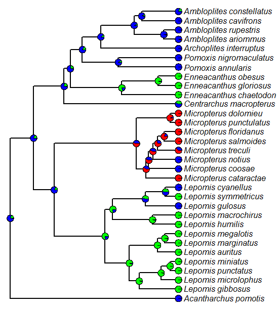
A phytools user contacted me to express difficulty in controlling pie colors at nodes using the new phytools functions for ancestral character estimation under the threshold model, ancThresh and plotThresh. This is done using the argument piecol, set to a vector with the states for the discrete trait as names, and the desired colors as values (in any format acceptable by R, e.g., here).

Here's a quick demo. I assume that we've already run the MCMC, and mcmc is the object returned by ancThresh. Data are in X:
> cols
   not     mod    high
"green"  "blue"   "red"
> plotThresh(tree,X,mcmc,piecol=cols,tipcol="estimated", label.offset=0.01)

Note that label.offset is on the scale of your phylogeny, so will have to be varied with total tree length. I've been meaning to migrate control of the pie sizes to the user, but have not yet had time to do so. (Plus, I've been sick.)

Two years of blogging

$
0
0
Just as the title of this post would suggest, phytools blog is two years old** today. (**More or less - as I noted last year, I had a few earlier placeholder posts, but my first serious entry was dated Dec. 24, 2010; and I first advertised this new blog via the now defunct dechronization blog the next day.)

In two years of blogging I have created over 320 posts. Obviously, some entries are very brief - maybe just a few words about a bug fix or report. In others, I was more in depth - for instance, when I wrote about the difficulty of estimating phylogenetic signal on very small trees; or when I discussed how to include fossil phenotypes in the estimation of ancestral states. If printed as a book (and, who knows, perhaps it will one day form the basis for one), the phytools blog would be a dense tome containing over 350 pages. Yikes!

The phytools blog has also grown in popularity over the past year. Raw "pageview" counts can be affected by many things, and are thus difficult to interpret, but phytools blog has received over 90,000 pageviews since it's creation - over 60,000 in the past year. By any measure, that rate is growing - and this also equates to over 160 pageviews/day for 2012. Among the posts accruing the greatest number of pageviews in 2012: my series on xkcd style trees (e.g., 1, 2, 3); my entries on visualizing trait evolution on trees using colors (e.g., 1, 2); and my posts about ancestral character estimation under the threshold model from quantitative genetics (e.g., 1, 2, 3).

The phytools package (also on CRAN) has grown as well. From a small hodgepodge of methods, phytools has grown into a big one - now containing over 80 different functions and a PDF manual that (as of latest CRAN release) contained 87 pages.

Towards the end of 2012, phytools blog got a new look. Since when the original visual theme was created, phytools had no plotting functions (but now it has tons), this seemed appropriate. The blog also got a new URL (after I obtained the domain phytools.org).

I don't doubt for a second that 2013 will be just as productive as 2012 - so thanks for reading, and please keep coming back. Happy holidays!

Processing .tps morphometric files in R

$
0
0
This has absolutely nothing to do with phylogenetics, but today (New Year's day 2013!) I've been starting the year with some R programming to pull data out of the raw output files from a program tpsDIG2 (by Jim Rohlf) that we use to get data from landmarks on digital skeletal x-rays of lizards.

We are just getting linear measurements at the moment (no fancy geometric morphometrics), so our data analysis is pretty simple. Here's what a skeletal x-ray of a lizard with the landmark coordinates overlain looks like (click for larger version):
(There is also a scale bar, not shown.)

The output from tpsDIG looks as follows (some lines omitted):
LM=43
726.00000 1580.00000
773.00000 1457.00000
679.00000 1456.00000
840.00000 1493.00000
840.00000 1463.00000
...
IMAGE=KMW_122_adj.tif
SCALE=0.125544

The first line gives the number of landmarks; subsequent lines give the horizontal & vertical pixel positions for each landmark; and the final lines give the image information & scale. Obviously, in R we want to read in the file, translate it to meaningful (i.e., non-pixel) scale, and perhaps compute our desired linear measurements. We might also want to be able to visually inspect our data for errors.

I have written two functions tps.process (to pull data out of the file and translate the scale); and tps.postProcess, which computes the linear measures we want from our input files. The first function is thus "general" (suitable for many people getting linear measures from .tps files); whereas the latter is specific to our data, although it could probably be modified and re-purposed easily. The code is posted here.

Here's a quick example. Note that I have also included a mode tps.process(...,type="anole") that visualizes the landmark data (for error checking) in a sensible way specifically for our x-rays.

> list.files()
[1] "KMW_004.tps" "KMW_122.tps" "KMW_317.tps"
[4] "tps.process.R"
> files<-list.files(pattern=".tps")
> files
[1] "KMW_004.tps" "KMW_122.tps" "KMW_317.tps"
> source("tps.process.R")
> X<-tps.process(files,type="anole")
OK? Press <Enter> to continue...
One of the plots above is created for each input .tps file so that we can easily review our input data for errors. (You can see it even looks kind of like a lizard!)

> # Here's our data rescaled
> X
$KMW_004adj
         V1        V2
1  28.338576 75.445244
2  33.807424 59.287284
3  21.751100 59.784452
4  49.343924 62.643168
5  47.355252 59.287284
6   6.214600 60.157328
...
$KMW_122_adj
         V1        V2
1  29.126208 80.724792
2  35.026776 65.282880
...
> # now let's automatically post-process
> LL<-tps.postProcess(X)
> LL
                rJL      lJL       JW    rMETC    lMETC
KMW_004adj  17.05837 16.98986 12.06657 3.900868 3.890955
KMW_122_adj 16.53086 16.64819 11.80180 3.766320 3.694494
KMW_317adj  15.80653 16.18932 11.41486 3.283738 3.391124
               rRAD     lRAD      rULN      lULN     rHUM
KMW_004adj  8.728803 8.672875  9.743256  9.175747 11.57585
KMW_122_adj 9.094794 9.109513 10.081895 10.313728 12.43139
KMW_317adj  8.239660 8.533229  9.663571  9.765426 12.13156
               lHUM     PECT     PELV     rFEM     lFEM
KMW_004adj  12.01011 8.082803 6.840578 16.44463 16.42960
KMW_122_adj 12.19394 7.910268 6.872889 17.09659 16.83975
KMW_317adj  11.85941 7.864227 6.990424 15.13729 15.12956
               rTIB     lTIB     rFIB     lFIB   rMETT1
KMW_004adj  13.59564 13.38724 13.41548 13.33405 5.133726
KMW_122_adj 14.58960 14.54415 14.47245 14.17035 5.280316
KMW_317adj  12.61329 12.73256 12.48540 12.61020 4.745144
             rMETT2   lMETT1   lMETT2
KMW_004adj  7.990535 4.991837 8.342392
KMW_122_adj 8.799730 5.176312 8.956841
KMW_317adj  7.743424 4.383258 7.899812

Now we have left & right measures for all the characters in our x-ray, above. Cool.

Adding new tips at random to a phylogeny

$
0
0
A friend and colleague contacted me recently with the request (somewhat abbreviated), below:

What I'm interested in doing is adding a given number of tips at random to a tree. I've done a comparison where I take a phylogeny. . . [and randomly prune taxa]. I'm interested to also do the reverse. . . . Would there be an easy way in phytools to do a "random addition of a given number of tips"?

Well, it is possible to randomly add tips to the tree - just by (for instance) picking nodes at random (from, say, the set of all internal & terminal nodes - excluding the root node), picking a position at random along the corresponding parent edge, and then using the phytools function bind.tip to attach the new tip to the tree.

So, for instance, we could just do:
> require(phytools)
> # simulate a random pure-birth tree
> tree<-pbtree(n=12)
> # pick a node at random
> node<-sample(c(1:length(tree$tip), 2:tree$Nnode+length(tree$tip)),size=1)
> node
[1] 22
> # pick a random position along the branch ending in node
> position<-runif(n=1)* tree$edge.length[which(tree$edge[,2]==node)]
> # this just tells us the relative position
> # (from the root)
> # check where the tip will be added
> (tree$edge.length[which(tree$edge[,2]==node)]- position)/tree$edge.length[which(tree$edge[,2]==node)]
[1] 0.700115
> # now attach new tip
> new.tree<-bind.tip(tree,"t13",where=node, position=position)
> # plot the trees
> par(mfrow=c(2,1))
> plotTree(tree,node.numbers=T)
> plotTree(new.tree,node.numbers=T)
We could do this sequentially a number of times - each time updating the tree as well as the set of nodes in the tree from which we are picking.

One shortcoming of this approach is that it ignores relative branch lengths - added tips are no more likely to be located on long branches than on short ones. Ideally, I think we'd like the probability of adding a tip along a branch to vary in direct proportion to the relative length of each branch. We can do that we taking advantage of the base function cumsum which (obviously) computes a cumulative sum from a vector. I have put this into a new function, add.random, which can be downloaded here. Let's test out the function to see if it behaves as we'd expect.
> source("add.random.R")
> # simulate a random, non-ultrametric tree
> tree1<-rtree(20)
> # set one branch to be very long (doesn't matter which)
> tree1$edge.length[sample(1:nrow(tree1$edge),size=1)]<-100
> # add new tips at random
> # here, we supply edge lengths - but we don't need to
> tree2<-add.random(tree1,n=10,edge.length=runif(n=10))
> # plot both trees
> layout(c(1,2),heights=c(2,3))
> plotTree(tree1,fsize=0.8)
> plotTree(tree2,fsize=0.8)
We can see that nearly all the new tips have been added on the very long branch that we created, which is exactly what we'd hoped.

As in the phytools function bind.tip, when the tree is ultrametric if new tips are added without branch lenghs, branch lengths are set such the tree remains ultrametric with the new tips. For example:
> # simulate pure-birth tree
> tree1<-pbtree(n=20)
> # add new tips at random, without supplying branch
> # lengths
> tree2<-add.random(tree1,n=10)
> # plot both trees
> layout(c(1,2),heights=c(2,3))
> plotTree(tree1,fsize=0.8)
> plotTree(tree2,fsize=0.8)
One thing that we can observe about the plots above is that because tips are added sequentially (not somehow all at once to the original tree), the resulting phylogeny can include entire clades (for instance, the group of ((t29,t25),t27)) not found in the original phylogeny.

Finally, we can also supply our own names, so, for instance:
> tree<-pbtree(n=12)
> tree<-add.random(tree,tips=c("huxley","darwin","wallace", "lyell"))
> plotTree(tree)
That's it!

New version of pgls.Ives

$
0
0
I just posted a new version of the phytools function pgls.Ives, which is a function to fit the regression model of Ives et al. (2007) incorporating sampling error in the estimation of species means (e.g., here).

The main update in this version is that it can now accept individual data, rather than just species means, variances, and covariances. The form for the individual data is the same as fitBayes (e.g., here) - in other words, just long vectors with names equal to the species names. Obviously, some names will repeat - which is allowed in vectors.

There is nothing magic about the way this function works. It just takes the individual data, and then computes the within-species variances and covariances (which are themselves used to estimate within-species sampling variances and covariances). This is done using, for example, R base functions such as aggregate. For those in need of a quick primer, the following demo shows how aggregate can be used to compute within-species variances and covariances for a vector of values x containing individual values with names(x) being the species names, some of which repeat:
> # simulate tree & data
> tree<-pbtree(n=30)
> x<-fastBM(tree) # true means
> # individual values
> xe<-sampleFrom(xhat,randn=c(1,5))
> xe
       t13         t13         t13         t13         t25
-1.83130612 -2.08011272 -1.99096486 -3.26950066 -1.17626558
       t25         t26         t26         t20         t20
0.57125210 -1.90520230 -1.96856340         ...         ...

> # get species means
> xbar<-aggregate(xe,by=list(names(xe)),FUN=mean)
> xbar<-setNames(xbar[,2],xbar[,1])
> xbar
        t1         t10         t11         t12         t13
-1.71666562 -3.92387486 -3.78403128 -1.82452852 -2.29297109
       t14         t15         t16         t17         t18
-0.83735741 -0.66027704 -1.84528088        ...         ...

> # get species variances
> xvar<-aggregate(xe,by=list(names(xe)),FUN=var)
> xvar<-setNames(xvar[,2],xvar[,1])
> xvar
        t1         t10         t11         t12         t13
0.319766112          NA 1.330431973 0.420867485 0.434420333
       t14         t15         t16         t17         t18
0.910668871 0.985273462 0.560029491        ...         ...


Something that's apparent from the little simulation above, is that if there is not at least two samples for a particular species, then the species variance cannot be computed. In that case, the program merely assumes that those species have within-species variance equal to the mean within-species variance - but it will also spit a warning to that effect.

Computing the sampling covariance from individual data requires that the same individuals be sampled in both vectors. Thus, if the argument Cxy is not supplied, pgls.Ives will try to do it. If different individuals were used for x&y, then sampling covariance is probably negligible. In this case - if individual data is being supplied - then one should also give the function a named vector of zeroes for the argument Cxy to avoid any errors of spurious results.

Finally, here's a quick demo showing how to use individual data with pgls.Ives for both zero and non-zero error covariance:
> # load source code
> source("pgls.Ives.R")

> # simulate tree & data under the regression model
> tree<-pbtree(n=30)
> xhat<-fastBM(tree)
> yhat<-0.75*xhat+0.2*fastBM(tree)

> # simulate individual data for x & y
> # assuming Cxy!=0
> x<-sampleFrom(xhat,randn=c(1,10))
> n<-summary(as.factor(names(x)))
> y<-sampleFrom(yhat,n=n[names(yhat)])

> # fit model
> pgls.Ives(tree,x,y)
$beta
[1] -1.193712  1.124268
$sig2x
[1] 0.5043893
$sig2y
[1] 0.219358
$a
[1] 3.111079 2.303972
$logL
[1] -74.45021
$convergence
[1] 0
$message
[1] "CONVERGENCE: REL_REDUCTION_OF_F <= FACTR*EPSMCH"

Warning messages:
1: Some species contain only one sample. Substituting mean variance.
2: Some species contain only one sample. Substituting mean variance.
3: Some species contain only one sample. Substituting mean variance.

Download the latest version of this function on the phytools page - or wait a bit and it will be in the next CRAN release.

Note on polytomies and internal branches of zero length in ancestral character estimation

$
0
0
Just a quick note on the use of polytomous trees vs. arbitrarily fully-resolved trees with branches of zero length in phytools functions for ancestral character estimation such as anc.Bayes, anc.ML, anc.trend, and ancThresh (as well as other actions that call these functions internally). Basically, and confusingly unlike functions such as pic in ape, polytomous trees (not internal branches of zero length) should be used. This is because of one specific internal calculation in these functions involving the inversion of the among tip species and internal node variance-covariance matrix computed by the phytools function vcvPhylo. If polytomies are represented using internal branches of zero length then vcvPhylo(tree) returns a singular matrix, which cannot be inverted. By contrast, if polytomies are represented as polytomies, vcvPhylo(tree) is not singular.

Here's an example:
> # create a tree with a polytomy
> tree<-read.tree(text="(A:2,(B:1,C:1,D:1):1);")
> plotTree(tree,node.numbers=TRUE)
> # compute among species & node VCV matrix
> C<-vcvPhylo(tree)
> C
 A B C D 6
A 2 0 0 0 0
B 0 2 1 1 1
C 0 1 2 1 1
D 0 1 1 2 1
6 0 1 1 1 1
> # invert?
> invC<-solve(C)
> invC # no problem
   A  B             C             D  6
A 0.5  0  0.000000e+00  0.000000e+00  0
B 0.0  1  0.000000e+00 -7.401487e-17 -1
C 0.0  0  1.000000e+00 -7.401487e-17 -1
D 0.0  0  4.163336e-17  1.000000e+00 -1
6 0.0 -1 -1.000000e+00 -1.000000e+00  4
> # resolve all nodes
> tree<-multi2di(tree)
> plotTree(tree,node.numbers=TRUE)
> # compute among species & node VCV matrix
> C<-vcvPhylo(tree)
> C
 A B C D 6 7
A 2 0 0 0 0 0
B 0 2 1 1 1 1
C 0 1 2 1 1 1
D 0 1 1 2 1 1
6 0 1 1 1 1 1
7 0 1 1 1 1 1
> # invert?
> invC<-solve(C)
Error in solve.default(C) :
Lapack routine dgesv: system is exactly singular: U[6,6]=0


It would seem to make sense to just include an internal step in all of these function in which we use di2multi to collapse any branches of zero length - the problem with this idea is that the consequence would be a disassociation between the node numbers of the original tree and the node numbers for which ancestral character estimates are returned. Yikes! In future versions of these functions I will try to remember to have them spit a meaningful error if a tree with branches of zero length is input - rather than just collapsing as at the present time.

A comment on the distribution of residuals (and data) for phylogenetic ANOVA

$
0
0
I get inquiries (with some regularity) about "testing for normality in phylogenetic (i.e., species) data" before phylogenetic regression or ANOVA; or about "satisfying the assumptions of parametric tests," by which is usually meant the assumption of normality.

I could probably write a whole paper about this (à la Revell 2009 or Revell 2010), but instead I'll make the simple point: we do not expect normality of the dependent (or independent, for continuous x) variables in phylogenetic data. Instead, what we do expect is multivariate normality of the residual error in y given X (or, equivalently, normality of y given X, controlling for the tree). This is actually a generally under-appreciated property of non-phylogenetic parametric statistical tests - but it is one that is entirely logical. Think: do we expect normality of human height, say, in order to fit an ANOVA model in which height depends on sex? Of course not, the response variable (height) is bimodal. ANOVA is appropriate to test for an effect of sex on height so long as the residual error in height controlling for sex is normal (and, like many such tests, may be fairly robust to mild violations of this assumption). Phylogenetic data are just a little more complicated because even after controlling for our main effects, the residual error can still be bi- or multi-modal due to phylogenetic correlations.

We can still test the parametric assumptions of our model - and I applaud those inclined to do so, as this is relatively seldom done in comparative studies. In the example below, I will first simulate data under the assumptions of the generalized phylogenetic ANCOVA; test normality of the response variable, y (it should fail) and my continuous covariate, x2 (it should fail); fit the phylogenetic ANCOVA model anyway, and then test normality of the residuals (these should fail, because the residuals are phylogenetically autocorrelated, see Revell 2009); mathematically "remove" the phylogeny, following Butler et al. (2000), and test for normality again (this time, it should pass). For normality testing, I'm using the Lilliefors (Kolmogorov-Smirnov) test, implemented in the R package nortest. A significant result means the data are not normally distributed.

> # load required packages
> require(phytools)
> require(nlme)
> require(nortest)
> # first simulate a completely balanced tree
> tree<-compute.brlen(stree(n=128,type="balanced"))
> # now simulate a discrete character on the tree
> Q<-matrix(c(-2,1,1,1,-2,1,1,1,-2),3,3)
> rownames(Q)<-colnames(Q)<-c(0,1,2)
> mtree<-sim.history(tree,Q)
> cols<-c("white","blue","red"); names(cols)<-0:2
> plotTree(mtree,ftype="off",lwd=5)
> plotSimmap(mtree,cols,pts=FALSE,ftype="off",lwd=3, add=TRUE)
This is the distribution of our effect on the tree.

> # now simulate data under an arbitrary ANCOVA model
> # the same principle applies to regression or ANOVA
> x1<-as.factor(mtree$states)
> x2<-fastBM(tree,sig2=2)
> e<-fastBM(tree)
> y<-2*as.numeric(x1)+0.75*x2+e
> # is y normal? (should fail)
> lillie.test(y)

       Lilliefors (Kolmogorov-Smirnov) normality test

data:  y
D = 0.1049, p-value = 0.00149

> # is x2 normal? (should fail)
> lillie.test(x2)

       Lilliefors (Kolmogorov-Smirnov) normality test

data:  x2
D = 0.1113, p-value = 0.0005154

> # fit the model
> fit<-gls(y~x1+x2,data=data.frame(x1,x2,y), correlation=corBrownian(1,tree))
> fit
Generalized least squares fit by REML
 Model: y ~ x1 + x2
 Data: data.frame(x1, x2, y)
 Log-restricted-likelihood: 40.7237

Coefficients:
(Intercept)         x11         x12          x2
 1.7388578   1.8929459   3.9681291   0.8418073

Correlation Structure: corBrownian
Formula: ~1
Parameter estimate(s):
numeric(0)
Degrees of freedom: 128 total; 124 residual
Residual standard error: 0.9261019
> # are the residuals normal? (should fail)
> lillie.test(residuals(fit))

       Lilliefors (Kolmogorov-Smirnov) normality test

data:  residuals(fit)
D = 0.1156, p-value = 0.0002458

> # are the residuals controlling for phylogeny normal?
> # (should pass)
> lillie.test(chol(solve(vcv(tree)))%*%residuals(fit))

       Lilliefors (Kolmogorov-Smirnov) normality test

data:  chol(solve(vcv(tree))) %*% residuals(fit)
D = 0.0694, p-value = 0.1371

The basic point is that we do not expect our input data in phylogenetic ANOVA or regression to be normally distributed - just the residual error controlling both for the main effects in our model, and (importantly, because this is most often forgotten) the tree.

Robinson-Foulds distance and NNI

$
0
0
A colleague just asked me:

Do you know of a way in R to calculate the topological difference between 2 trees as the (ed. minimum) number of nearest-neighbor interchanges required to go from one to the other?

I told him that I'm not sure of the reference for this, but if I remember correctly it is just the Robinson-Foulds distance divided by 2. Indeed, this seems to be the case. Below, I'll demo this. I first simulate a very large tree (I'll explain why in a moment), apply random NNIs using 'phangorn' function rNNI, and then compute RF distance for each tree (using phangorn::RF.dist). Here is the result:

> require(phangorn)
> tree<-rtree(n=10000)
> # one random NNI step
> trees<-rNNI(tree,moves=1,n=20)
> rf<-sapply(trees,RF.dist,tree2=tree)
> rf
[1] 2 2 2 2 2 2 2 2 2 2 2 2 2 2 2 2 2 2 2 2
> # two steps
> trees<-rNNI(tree,moves=2,n=20)
> rf<-sapply(trees,RF.dist,tree2=tree)
> rf
[1] 4 4 4 4 4 4 4 4 4 4 4 4 4 4 4 4 4 4 4 4
> # four steps
> trees<-rNNI(tree,moves=4,n=20)
> rf<-sapply(trees,RF.dist,tree2=tree)
> rf
[1] 8 8 8 8 8 8 8 8 8 8 8 8 8 8 8 8 8 8 8 8
> # 10 steps
> trees<-rNNI(tree,moves=10,n=20)
> rf<-sapply(trees,RF.dist,tree2=tree)
> rf
[1] 20 20 20 20 20 20 20 20 20 20 20 20 20 20 20 20 20 20
[19] 20 20
> # 20 steps > trees<-rNNI(t
ree,moves=20,n=20)
> rf<-sapply(trees,RF.dist,tree2=tree)
> rf
[1] 40 40 40 40 40 40 40 40 40 40 40 40 40 40 40 40 40 40
[19] 40 40

The reason I used a very large starting tree (10,000 tips in this case) was because for small trees, successive random NNIs will cancel each other with some regularity - making the minimum number of NNIs separating two trees (i.e., RF/2) smaller than the number of simulated NNIs. For example:

> tree<-rtree(n=50)
> # four steps
> trees<-rNNI(tree,moves=4,n=20)
> rf<-sapply(trees,RF.dist,tree2=tree)
> rf
[1] 8 8 4 6 8 8 8 8 8 8 8 8 8 8 8 8 8 8 8 8
> # 10 steps
> trees<-rNNI(tree,moves=10,n=20)
> rf<-sapply(trees,RF.dist,tree2=tree)
> rf
[1] 16 20 20 20 18 16 20 20 20 14 20 20 16 16 20 18 20 20
[19] 14 18
> # 20 steps
> trees<-rNNI(tree,moves=20,n=20)
> rf<-sapply(trees,RF.dist,tree2=tree)
> rf
[1] 26 20 22 26 32 28 32 28 34 34 28 24 30 32 34 24 30 38
[19] 26 34

This will eventually even happen for large trees. For fun, here is the some simulation code to compute the relationship between mean RF distance and number of random NNIs for trees of varying size:

# function to simulate rNNIs and return mean RF dist
f1<-function(tree,moves,n=20)
  mean(sapply(rNNI(tree,moves,n),RF.dist,tree2=tree))
# function to get the mean RF distance over random trees
f2<-function(moves,ntaxa,nrep=20,nmoves=20)
  mean(sapply(rmtree(N=nrep,n=ntaxa),f1,moves=moves, n=nmoves))
# now compute mean RF distance for various NNIs
# across trees of different size
moves<-c(2*1:5,15,20,30,40)
ntaxa<-c(10,20,40,80,160,320)
XX<-matrix(NA,length(moves),length(ntaxa), dimnames=list(moves,ntaxa))
for(i in 1:length(ntaxa))
  XX[,i]<-sapply(moves,f2,ntaxa=ntaxa[i])
# plot
plot(c(0,max(moves)),c(0,2*max(moves)),xlab="NNI moves", ylab="mean RF distance",type="l",lty=2, xlim=c(0,max(moves)+0.1*max(moves)),ylim=c(0,2*max(moves)))
for(i in 1:ncol(XX)){
  lines(moves,XX[,i],type="b")
  text(x=moves[length(moves)],y=XX[length(moves),i], paste("N=",ntaxa[i],sep=""),pos=4,offset=0.3)
}

If any readers know of the reference or proof for this - please post to the comments. (I only did a very casual search for this - it may be an easy reference to find, in which case I apologize.)

Reordering the columns of $mapped.edge for a set of stochastically mapped trees

$
0
0
I recently got the following comment to a recent post on the blog:

I am trying to play with your make.simmap function, but I found that in all the simulations, colnames(tree$mapped.edge) show a different order. This is problematic when I want to combine the results for models fitted over the multiples trees as done for instance with OUwie package.

It is true that the column order of $mapped.edge may differ in different mapped stochastic character histories. The matrix $mapped.edge is a matrix containing (in each row) the total time spent in each state (in columns) for a stochastic-map style tree stored by read.simmap or created by (for instance) make.simmap or sim.history. (The specific sequence and time spent in each state along each branch is stored in a separate component of the simmap object, a list called $maps).

The matrix $mapped.edge exists primarily to serve downstream functions, such as brownie.lite or evol.vcv for which the only attribute that's important about the mapping is the time spent in each state on each edge, regardless of the ordering.

The fact that the column orderings can be different in a set of mappings is not an oversight. I at some point made the arbitrary decision that the column order of $mapped.edge should be the order in which the discrete trait appears in the tree - from the root forwards through my upward tree traversal algorithm. Thus the first column of $mapped.edge will always be the discrete state mapped to the root of the tree in question - but the second column will be determined based on both the height and position in the tree, relative to my traversal path from the root to the tips.

I decided to use this ordering instead of, say, the alphabetical or numerical order of the mapped discrete character states because we are not assuming any natural ordering for the trait.

I feel nearly certain that in a prior post I have addressed how to reorganize the output of, say, brownie.lite to average the estimated rates from different mappings across mapping in which the columns of $mapped.edge (and thus the output order of the rates) differ among trees. However, an alternative is to reorder the columns of each matrix $mapped edge in each tree object prior to analysis. Here is an illustration of the "problem" and the code to fix it:

> # load phytools
> require(phytools)
> # ok lets simulate some data to illustrate the problem
> Q<-matrix(c(-2,1,1,1,-2,1,1,1,-2),3,3)
> rownames(Q)<-colnames(Q)<-c("A","B","C")
> tree<-pbtree(n=100,scale=1)
> # our discrete character
> X<-sim.history(tree,Q)$states
> # our stochastically mapped trees
> mtrees<-make.simmap(tree,X,nsim=100)
> cols<-c("red","blue","green"); names(cols)<-c("A","B","C")
> layout(matrix(1:100,10,10))
> plotSimmap(mtrees,cols,ftype="off",pts=FALSE)
Waiting to confirm page change...

We can see from this plot that at, although the majority of trees appear to have state "B" (blue) as the root state, at least trees 1, 3, and 4 (among others) have different root node states and thus will have different orderings of the matrix $mapped.edge. Let's confirm this:
> mtrees[[1]]$mapped.edge
        state
                   C            A            B
 101,102 0.101357902 5.474078e-05 0.0000000000
 102,103 0.000000000 2.644562e-01 0.0000000000
 103,104 0.007755547 2.602131e-01 0.0000000000
 104,1   0.340476206 2.568633e-02 ...
 ...
> mtrees[[3]]$mapped.edge
        state
                    A            B            C
 101,102 0.1014126423 0.0000000000 0.0000000000
 102,103 0.2644561833 0.0000000000 0.0000000000
 103,104 0.1063332481 0.1616353949 0.0000000000
 104,1   0.0000000000 0.2404987635 ...
 ....
> mtrees[[4]]$mapped.edge
        state
                    B           A            C
 101,102 0.1014126423 0.000000000 0.0000000000
 102,103 0.2644561833 0.000000000 0.0000000000
 103,104 0.1886379373 0.079330706 0.0000000000
 104,1   0.0000000000 0.102319207 ...
 ....

Ok - now let's try sorting the columns of $mapped.edge. Note that no downstream functions (in phytools, at least) that use this style of tree assume any specific ordering for the columns of $mapped.edge, so this change should not affect the function of the object.

Here's our code (modify as appropriate):
# pick an ordering
# (this could also be the ordering of e.g. the first tree)
ordering<-c("A","B","C")
# function to reorder
foo<-function(tree,ordering){
  tree$mapped.edge<-tree$mapped.edge[,ordering]
  tree
}
# apply to all trees
mtrees<-lapply(mtrees,foo,ordering=ordering)
class(mtrees)<-"multiPhylo"

Now let's check our three trees from before:
> mtrees[[1]]$mapped.edge
        state
                    A            B           C
 101,102 5.474078e-05 0.0000000000 0.101357902
 102,103 2.644562e-01 0.0000000000 0.000000000
 103,104 2.602131e-01 0.0000000000 0.007755547
 104,1   2.568633e-02 0.0000000000 ...
 ....
> mtrees[[3]]$mapped.edge
        state
                    A            B            C
 101,102 0.1014126423 0.0000000000 0.0000000000
 102,103 0.2644561833 0.0000000000 0.0000000000
 103,104 0.1063332481 0.1616353949 0.0000000000
 104,1   0.0000000000 0.2404987635 ...
 ....
> mtrees[[4]]$mapped.edge
        state
                   A            B            C
 101,102 0.000000000 0.1014126423 0.0000000000
 102,103 0.000000000 0.2644561833 0.0000000000
 103,104 0.079330706 0.1886379373 0.0000000000
 104,1   0.102319207 0.0000000000 ...
 ....

Good, it works. (Note that we could have also just as easily done this with a simple for loop.)

Addendum to the relationship between NNIs and Robinson-Foulds distance

$
0
0
In a previous post I commented that, for a broad range of trees and simulated NNIs, the minimum number of NNIs to get between two topologies seemed to be equal to (one half) the Robinson-Foulds distance. I asked readers of this blog if they were aware of any citations for this general property.

Well, it turns out that a reader responded, and RF distance does not give us (two times) the minimum number of NNIs to get between topologies - and, furthermore, computing the actual NNI distance is NP-hard. Rather, RF distance could be said to be a lower bound on the minimum number of NNIs to get between topologies. In other words, it cannot take fewer than (one half) the RF distance NNIs to get between two topologies - but it can take more. The commenter (Leonardo de Oliveira Martins from the University of Vigo, Spain) even wrote a very nice post on his own blog explaining why this is the case.

Very cool.

New version of phytools (0.2-16)

$
0
0
I just posted a new, non-CRAN phytools version (0.2-16). There are not a huge number of updates in this version from the last non-CRAN phytools version (0.2-15), but the updates since the last CRAN release (2012-11-13) are considerable. I plan to submit a new version to CRAN soon. Here is a list of updates in this version relative to phytools 0.2-15:

1. An updated version of pgls.Ives that can (optionally) compute sampling variances and covariances for species means internally.

2. A new function, add.random, which can add new tips at random to a tree (and also assign branch lengths to keep an ultrametric tree ultrametric, which is neat).

3. A new utility function, orderMappedEdge, which sorts the column order of $mapped.edge in a "multiPhylo" set of phylogenies with mapped discrete traits.

Finally, 4. updates to anc.ML, ancThresh, anc.trend, and anc.Bayes, to return a sensible error if internal or terminal branches of zero length will cause analyses to fail. Note that fastAnc, because it uses contrasts to get the ML ancestral states, needs a fulling bifurcating tree - although it can also convert the tree internally and then backtranslate the node IDs.

I think that covers everything.

As usual, you can download this version here and install from source:
> install.packages("phytools_0.2-16.tar.gz",type="source", repos=NULL)
* installing *source* package 'phytools' ...
** R
...

* DONE (phytools)

Please let me know if you find any bugs!

New version of function for MRP supertree estimation

$
0
0
I just posted a new version of the phytools function mrp.supertree for supertree estimation via Matrix Representation Parsimony (MRP). The main update for the user is that now control of optimization, which is performed by functions in the phangorn package, have been migrated to the user. That means that the parsimony optimization can be performed using optim.parsimonyorpratchet, and all the options in both of these functions can now be controlled by the user (without having to, say, modify the source code of mrp.supertree). Note that the options of optim.parsimony and pratchet have changed relatively recently, particularly the types of tree rearrangements that are possible during tree search - so users should make sure that the have the latest version of phangorn (and its dependencies, which include a very recent version of ape) installed.

The function works OK - but I offer two points of caution. One, optimization via optim.parsimony and pratchet, even using SPR for tree rearrangements, is not terrific. This can be determined by comparing optimization from a random starting tree to optimization when the true tree is provided as a starting tree. I would recommend running the function multiple times with different or random starting trees to evaluate convergence. Two, the internally called parsimony optimizers are also a little buggy. In my experience they sometimes quit unexpectedly or cause R to crash. I'm sure that Klaus is working on this.

The updated code for this function is here. I will also plan to post more about this later.

More on MRP supertree estimation in phytools

$
0
0
In a post from earlier today, I described some of the updates in a new version of the phytools function mrp.supertree. The two main changes are as follows: (1) now the user can decide which parsimony optimization method (optim.parsimony or pratchet) is called inside the function; and (2) now near total control of the optimizer has been transferred to the user.

What this means is that (with one exception*) all the options of optim.parsimony and pratchet (summarized here) can now be controlled by the user. The exception is really only a modification to how the optimizer is controlled. For mrp.supertree(...,method="optim.parsimony") the argument start is substituted for the argument tree in optim.parsimony; and, for both mrp.supertree(...,method="pratchet") and mrp.supertree(...,method="optim.parsimony"), the argument start can be an object of class "phylo", i.e., a true starting tree, or, it can be a method for obtaining the starting tree - where the options are start="NJ" or start="random". For start="NJ" we first compute the neighbor-joining tree from the distances in the MRP trees matrix. I can't justify this theoretically, but it does seem to put us in the neighborhood of the MRP MP tree more effectively than random chance.

I thought I'd just show a quick demo of how the new version of mrp.supertree can be used - as well as how bad it can be under some circumstances. One good thing about the modifications I've made to the function is that now it will more easily inherit any additional improvements Klaus makes to the optimizers in the phangorn package.

> # load phytools & source
> require(phytools)
> source("mrp.supertree.R")
> # simulate a tree
> tree<-rtree(n=100,rooted=FALSE)
> # function randomly subsamples a tree to n species
> foo<-function(x,n){
+ tips<-sample(x$tip.label)[1:n]
+ x<-drop.tip(x,setdiff(x$tip.label,tips))
+ }
> # generate a set of subsampled trees
> trees<-replicate(n=5,foo(tree,40),simplify=FALSE)
> class(trees)<-"multiPhylo"
> # now I have 5 trees subsampled differently from the same
> # parent tree
> # attempt supertree estimation
> st.nni<-mrp.supertree(trees) # default method
[1] "Best pscore so far: 289"
[1] "Best pscore so far: 289"v [1] ...
pratchet() found 5 supertrees
with a parsimony score of 285 (minimum 185)
> # SPR tree rearrangment
> st.spr<-mrp.supertree(trees,rearrangements="SPR")
[1] 288
[1] ...
[1] "Best pscore so far: 202"
[1] ...
The MRP supertree, optimized via pratchet(),
has a parsimony score of 202 (minimum 185)
> # SPR with a better starting tree
> st.nj<-mrp.supertree(trees,rearrangements="SPR", start="NJ")
[1] "Best pscore so far: 332"
[1] ...
The MRP supertree, optimized via pratchet(),
has a parsimony score of 199 (minimum 185)
> # optim.parsimony with SPR
> st.op<-mrp.supertree(trees,rearrangements="SPR", method="optim.parsimony",start="NJ")
[1] 288
[1] ...
Final p-score 202 after 37 nni operations
The MRP supertree, optimized via optim.parsimony(),
has a parsimony score of 202 (minimum 185)
> # ok, now as a check let's try with the true tree
> # as our starting tree
> # (we have to prune some tips that were not in our sampled trees)
> tips<-unique(as.vector(sapply(trees,function(x) x$tip.label)))
> st.tt<-mrp.supertree(trees,method="optim.parsimony", start=drop.tip(tree,setdiff(tree$tip.label,tips)))
Final p-score 185 after 0 nni operations
The MRP supertree, optimized via optim.parsimony(),
has a parsimony score of 185 (minimum 185)
> # obviously we didn't do so hot before, but let's verify
> # first compute the tree containing only subsampled tips
> sub<-drop.tip(tree,setdiff(tree$tip.label,tips))
> sapply(st.nni,dist.topo,sub)
[1] 140 140 140 140 140
> dist.topo(st.spr,sub)
[1] 82
> dist.topo(st.nj,drop.tip(tree,sub)
[1] 80
> dist.topo(st.op,sub)
[1] 82
> # as a check
> dist.topo(st.tt,sub)
[1] 0

This suggests to me that we have enough information in our input trees to get our true tree back (at least for the tips we sampled) - but due to limits on optimization, as far as it has been implemented so far - we're just not getting there.

For comparison, we could try a similar example in which we subsample a much larger fraction of the taxa in each tree - say 60% instead of 40%:

> # generate a set of subsampled trees
> trees<-replicate(n=5,foo(tree,60),simplify=FALSE)
> class(trees)<-"multiPhylo"
> # now I have 5 trees subsampled differently from the same
> # parent tree
> st.nni<-mrp.supertree(trees)
...
The MRP supertree, optimized via pratchet(),
has a parsimony score of 376 (minimum 285)
> st.spr<-mrp.supertree(trees,rearrangements="SPR")
...
The MRP supertree, optimized via pratchet(),
has a parsimony score of 285 (minimum 285)
> st.nj<-mrp.supertree(trees,rearrangements="SPR", start="NJ")
...
The MRP supertree, optimized via pratchet(),
has a parsimony score of 285 (minimum 285)
> st.op<-mrp.supertree(trees,rearrangements="SPR", method="optim.parsimony",start="NJ")
...
Final p-score 285 after 49 nni operations
The MRP supertree, optimized via optim.parsimony(),
has a parsimony score of 285 (minimum 285)
> st.tt<-mrp.supertree(trees,method="optim.parsimony", start=tree)
Final p-score 285 after 0 nni operations
The MRP supertree, optimized via optim.parsimony(),
has a parsimony score of 285 (minimum 285)
> dist.topo(st.nni,tree)
[1] 92
> dist.topo(st.spr,tree)
[1] 14
> dist.topo(st.nj,tree)
[1] 14
> dist.topo(st.op,tree)
[1] 14
> dist.topo(st.tt,tree)
[1] 0

No huge surprise that we do much better when we have more data. Something that is notable is that even though we get a "perfect score," so to speak, in all runs except for the default - there is still some topological discordance between the supertrees and the true trees. Most likely this is because some splits are not found in any of the trees used for supertree estimation. Effectively, heuristic parsimony searching will find just one of the possible resolutions of the true uncertainty about this node. The consequence - topological discordance between the estimated and the true trees.

Updated phylANOVA

$
0
0
A user phytools user recently contacted me with the bug report that for a tree with multifurcations they received the following error from the function phylANOVA:
Error in pic(y, tree) : 'phy' is not rooted and fully dichotomous

phylANOVA is a function that does the simulation-based phylogenetic ANOVA of Garland et al. (1993), but with posthoc tests about the group means - also based on simulation. (Note that this is the same as the "geiger" function phy.anova, but with the posthoc comparison of means added in.)

There's no inherent reason why the function should require a fully bifurcating tree. The reason that it does is because I use pic as a quick way to compute the Brownian motion rate of evolution for simulation, and pic needs a binary tree as input. This bug is easily fixed.

I've updated the code. The link to the new code is here. The following shows a simulation of a tree with multifurcations and data for the phylogenetic ANOVA; a failed analysis with the current version of the code; and a successful analysis with the updated version. Note that there are some neat tricks of simulation thrown in here....

> # load phytools
> require(phytools)
> # simulate tree
> tree<-pbtree(n=50)
> # set some branches to zero to create polytomies
> tree$edge.length[tree$edge.length<0.1]<-0
> is.ultrametric(tree) # check if ultrametric
[1] FALSE
> # now add some length to terminal branches so that
> # the tree is ultrametric
> addTip<-max(vcv(tree))-diag(vcv(tree))
> tree$edge.length[tree$edge[,2]<=length(tree$tip)]<- tree$edge.length[tree$edge[,2]<=length(tree$tip)]+addTip
> tree<-di2multi(tree)
> is.ultrametric(tree) # check if ultrametric
[1] TRUE
> is.binary.tree(tree) # check if bifurcating
[1] FALSE
> # let's take a look at our tree with polytomies
> plotTree(tree,fsize=0.8)
> # ok now let's create a discrete character on the tree
> Q<-matrix(c(-2,1,1,1,-2,1,1,1,-2),3,3)
> rownames(Q)<-colnames(Q)<-c("A","B","C")
> x<-sim.history(tree,Q)$states
> # now let's add an effect that depends on the tip state
> # for the discrete trait
> X<-sapply(c("A","B","C"),"==",x)*1
> y<-X%*%c(0,2,6)+fastBM(tree)
> # conduct phylogenetic ANOVA (current function)
> phylANOVA(tree,x,y) # fails
Error in pic(y, tree) : 'phy' is not rooted and fully dichotomous
> # with a multi2di resolved tree
> phylANOVA(multi2di(tree),x,y)
$F
[1] 10.11326
$Pf
[1] 0.003
$T
        A         B         C
A 0.000000 -1.514359 -4.496845
B 1.514359  0.000000 -2.618537
C 4.496845  2.618537  0.000000
$method
[1] "holm"
$Pt
     A     B     C
A 1.000 0.185 0.003
B 0.185 1.000 0.006
C 0.003 0.006 1.000

> # load updated version
> source("phylANOVA.R")
> phylANOVA(tree,x,y)
$F
[1] 10.11326
$Pf
[1] 0.001
$T
        A         B         C
A 0.000000 -1.514359 -4.496845
B 1.514359  0.000000 -2.618537
C 4.496845  2.618537  0.000000
$method
[1] "holm"
$Pt
     A     B     C
A 1.000 0.172 0.003
B 0.172 1.000 0.014
C 0.003 0.014 1.000

Fix to fastAnc

$
0
0
A colleague recently reported bad behavior in the fast ancestral character estimation function fastAnc that he hypothesized was due to the fact that I extracted the total number of tips in the tree using the shorthand N<-length(tree$tip) in place of N<-tree$tip.label. In principle this shouldn't be a problem because list elements, unlike variables, can be called by any unambiguous abbreviation of the element name (that is, if we use the $ operator - see below).

So, for instance:
> exampleList<-list(x=c(1,2),test=c("A","B","C"))
> exampleList$t
[1] "A" "B" "C"
> exampleList$test2<-c("D","E","F")
> exampleList$t # no longer umambiguous
NULL
> exampleList$test
[1] "A" "B" "C"

As an aside, if we want to call elements in a list accepting only an exact match the name, then we have to use [[ instead of $. So, for instance:
> exampleList$test2<-NULL
> exampleList$t
[1] "A" "B" "C"
> exampleList[["t"]]
NULL
> exampleList[["test"]]
[1] "A" "B" "C"
> # tell R to allow partial match
> exampleList[["t",exact=FALSE]]
[1] "A" "B" "C"

This is the reason why either:
> tree<-pbtree(n=112)
> length(tree$tip)
[1] 112
> # or
> length(tree$tip.label)
[1] 112
will, generally speaking, serve equally well in computing the number of tips in a tree.

However, what the exercise above inadvertently shows is that if we were to create a custom "phylo" object (which we have every right to do), we could do so by adding an additional list component, for instance $tip.states. If we did, it could create confusion when we compute the number of terminal species in the tree using length(tree$tip). So, for instance:
> x<-fastBM(tree)
> tree$tip.states<-x
> length(tree$tip)
[1] 0
> length(tree$tip.label)
[1] 112

This suggests that it might not be the best programming practice to assume that length(tree$tip) will invariably compute the number of species in the tree. I have updated fastAnc, here, but I know for a fact that this kind of code shorthand exists in other functions of the phytools package as well. I will try to update these as time goes on.

BTW - in that example with the custom element $tip.states, here is what fastAnc does:
> fastAnc(tree,x)
Error in root(btree, node = i) :
 incorrect node#: should be greater than the number of taxa
> # load the updated source
> source("fastAnc.R")
> fastAnc(tree,x)
       113         114         115  ...
-0.59341281 -0.03688321  0.89743347  ...
Viewing all 802 articles
Browse latest View live