I just updated the phytools function phylo.to.map (or, more accurately, the phytools S3 method for objects of class "phylo.to.map") to permit the use of ape functions nodelabels, tiplabels, etc., by assigning the environmental variable "last_plot.phylo".

Here's a quick demo using some very simple simulated data:

## first install the latest version from GitHub
library(devtools)
install_github("liamrevell/phytools")

library(phytools)
## simulate tree & data
tree<-pbtree(n=26,scale=100,tip.label=LETTERS)
lat<-fastBM(tree,sig2=10,bounds=c(-90,90))
long<-fastBM(tree,sig2=80,bounds=c(-180,180))
obj<-phylo.to.map(tree,cbind(lat,long))

## objective: 108
## objective: 108
## objective: 108
## objective: 108
## objective: 108
## objective: 108
## objective: 104
## objective: 104
## objective: 104
## objective: 94
## objective: 94
## objective: 88
## objective: 88
## objective: 86
## objective: 84
## objective: 84
## objective: 84
## objective: 82
## objective: 82
## objective: 82
## objective: 82
## objective: 82
## objective: 82
## objective: 82
## objective: 80

## add nodelabels
nodelabels()

Note that if rotate=TRUE in phylo.to.map (the default) the tree may have been rotated and consequently the node labels may not match the node indices in the original input tree!

Here's another example of a use:

obj

## Object of class "phylo.to.map" containing:
## 
## (1) A phylogenetic tree with 26 tips and 25 internal nodes.
## 
## (2) A geographic map with range:
##      -85.19N, 83.6N
##      -180W, 180W.
## 
## (3) A table containing 26 geographic coordinates.

par(fg=grey(0.4))
plot(obj,colors="black",ftype="off",lwd=1,lty="dotted",ylim=c(-90,100))
tiplabels(pch=19,col="red")
points(obj$coords[,2:1],col="red",pch=19)

Or something like this. Well, at least it adds some flexibility.

A recent R-sig-phyo user reported a problem with describe.simmap in phytools when trying to use it to summary the results from stochastic mapping across multiple trees with potentially incongruent topologies. This is unsurprising to me because the method is not intended for use with such a set of trees - and it assumes, in fact, that all trees are identical. (It does not check for this by default since this is quite slow - but this is an option is check.equal is set to TRUE.)

For a while, however, I have been meaning to update the function to be able to handle trees with incongruent topologies - by, for example, matching nodes across trees & then only computing the frequency of being in each state for nodes present in the consensus topology or a reference tree.

I just posted exactly this update; however users are cautioned that this has not yet been thoroughly tested. Here is a quick demo:

library(devtools)
install_github("liamrevell/phytools")

## load packages
library(phytools)
## here are our trees:
trees

## 100 phylogenetic trees with mapped discrete characters

## they are incongruent:
par(mfrow=c(10,10))
colors<-setNames(c("blue","red"),c("a","b"))
plot(trees,lwd=1,ftype="off",colors=colors)

OK, now let's use the method. First, without checking for equality:

obj<-summary(trees)
obj

## 100 trees with a mapped discrete character with states:
##  a, b 
## 
## trees have 41.23 changes between states on average
## 
## changes are of the following types:
##        a,b   b,a
## x->y 19.51 21.72
## 
## mean total time spent in each state is:
##               a          b    total
## raw  15.1882814 11.8398964 27.02818
## prop  0.5619425  0.4380575  1.00000

plot(obj,colors=colors)
add.simmap.legend(colors=colors,x=5,y=3,prompt=FALSE)

It may not be completely obvious - but close examination reveals that this is not a good result. For instance - tip states do not even necessarily match the input values:

x

##   A   F   P   K   T   W   U   Y   N   V   J   S   H   C   E   D   L   R 
## "b" "a" "a" "b" "b" "a" "b" "a" "a" "a" "a" "b" "b" "a" "a" "a" "a" "a" 
##   X   M   B   G   Q   Z   O   I 
## "b" "a" "a" "a" "b" "a" "b" "a"

OK, now let's check if the trees are equal. In the new phytools version of this function when trees are not equal, a consensus tree is built which is then used to compute posterior probabilities for nodes (that occur in the consensus tree). Of course, we will lose our branch lengths:

obj<-summary(trees,check.equal=TRUE) ## much slower

## Note: Some trees are not equal.
## A "reference" tree will be computed if none was provided.
## 
## No reference tree provided & some trees are unequal.
## Computing majority-rule consensus tree.

obj

## 100 trees with a mapped discrete character with states:
##  a, b 
## 
## trees have 41.23 changes between states on average
## 
## changes are of the following types:
##        a,b   b,a
## x->y 19.51 21.72
## 
## mean total time spent in each state is:
##               a          b    total
## raw  15.1882814 11.8398964 27.02818
## prop  0.5619425  0.4380575  1.00000

plot(obj,colors=colors)
add.simmap.legend(colors=colors,x=0,y=3,prompt=FALSE)

Finally, if we have some kind of pre-existing reference tree, such as (for example) a Bayesian MCC tree, and we want to input it & compute Bayesian posterior probabilities on that tree, we can do it:

tree

## 
## Phylogenetic tree with 26 tips and 25 internal nodes.
## 
## Tip labels:
##  A, F, P, K, T, W, ...
## 
## Rooted; includes branch lengths.

obj<-summary(trees,ref.tree=tree)
obj

## 100 trees with a mapped discrete character with states:
##  a, b 
## 
## trees have 41.23 changes between states on average
## 
## changes are of the following types:
##        a,b   b,a
## x->y 19.51 21.72
## 
## mean total time spent in each state is:
##               a          b    total
## raw  15.1882814 11.8398964 27.02818
## prop  0.5619425  0.4380575  1.00000

plot(obj,colors=colors)
add.simmap.legend(colors=colors,x=4.5,y=3,prompt=FALSE)

That's it!

As warned, I just did this - so there are sure to be bugs. Please report any via email or on R-sig-phylo. Thanks!

I just added a function to phytools to automate the task of attaching species-level subtrees simulated under a Yule process to a backbone genus-level tree. I described this here last week.

Here is how it works:

## first update phytools
library(devtools)
install_github("liamrevell/phytools")

## load
library(phytools)
## here's our hypothetical genus tree:
genus.tree

## 
## Phylogenetic tree with 16 tips and 15 internal nodes.
## 
## Tip labels:
##  Vkfns, Ikfxnyht, Qkyca, Bnlpd, Wkpws, Bkhq, ...
## 
## Rooted; includes branch lengths.

plotTree(genus.tree,ftype="i")

## here are our tips to add
tips

##  [1] "Ikfxnyht_opqcfh" "Ikfxnyht_nvaocw" "Ikfxnyht_knzcyf"
##  [4] "Qkyca_pzdukv"    "Qkyca_jukdfi"    "Qkyca_ritdjl"   
##  [7] "Qkyca_agrjou"    "Qkyca_qoyafl"    "Qkyca_qrfsbu"   
## [10] "Bnlpd_hidqnw"    "Bnlpd_wlthqi"    "Bnlpd_gayokd"   
## [13] "Bnlpd_lqjspu"    "Wkpws_xbahqo"    "Wkpws_pwdnuv"   
## [16] "Bkhq_hqdkbx"     "Bkhq_ojrbaw"     "Bkhq_pzwyfq"    
## [19] "Bkhq_dejpxs"     "Bkhq_efnyzp"     "Bkhq_kymfvj"    
## [22] "Bgln_tfuizj"     "Bgln_tpdsuf"     "Bgln_ycaqrs"    
## [25] "Bgln_havrzp"     "Bgln_bonyms"     "Bgln_nhquvm"    
## [28] "Nrztfp_blunwa"   "Iakywem_jqhxdr"  "Lhkrtyl_usqjhl" 
## [31] "Lhkrtyl_nbjhyc"  "Lhkrtyl_wmhkcd"  "Lhkrtyl_wmdkqp" 
## [34] "Lhkrtyl_dfhlkj"  "Lhkrtyl_kpadxb"  "Javcgbph_qvgmrh"
## [37] "Javcgbph_vzqfir" "Ctfioy_yjuxhp"   "Ctfioy_bcgonv"  
## [40] "Yrvp_prchgs"     "Yrvp_zcjuqx"     "Yrvp_usjbyc"    
## [43] "Hmvlk_nymqow"    "Hmvlk_ktjxnq"    "Hmvlk_crtdau"   
## [46] "Hmvlk_hemxwi"    "Hmvlk_xygpmk"    "Hmvlk_hxofgw"   
## [49] "Fioxrcyl_pecahk" "Fioxrcyl_uifsdv" "Okmfyg_ahxljq"

## add them:
species.tree<-genus.to.species.tree(genus.tree,tips)
plotTree(species.tree,ftype="i",fsize=0.7)

That's it.

Obviously, the data & tree above were simulated. Here is code used in simulation

## first let's simulate our genus tree:
foo<-function() paste(sample(LETTERS,1),paste(sample(letters,
    round(runif(1,min=3,max=7))),collapse=""),sep="")
genera<-replicate(16,foo())
genus.tree<-pbtree(n=length(genera),tip.label=genera,scale=80)
genus.tree$edge.length[which(genus.tree$edge[,2]<=Ntip(genus.tree))]<-
    genus.tree$edge.length[which(genus.tree$edge[,2]<=Ntip(genus.tree))]+20
tips<-c()
for(i in 1:Ntip(genus.tree)){
    n.genus<-sample(0:6,1)
    if(n.genus>0) for(j in 1:n.genus) 
        tips<-c(tips,paste(genus.tree$tip.label[i],
        paste(sample(letters,6),collapse=""),sep="_"))
}

I recently made a couple of small updatesto plotSimmap - firstly, to allow user control of the line end type (lend, as in par); and secondly, for type="fan", to plot the two edges originating from the root as a single segmented line.

Here is a quick example using the latest version of phytools on GitHub:

library(phytools)
packageVersion("phytools")

## [1] '0.5.59'

data(anoletree)
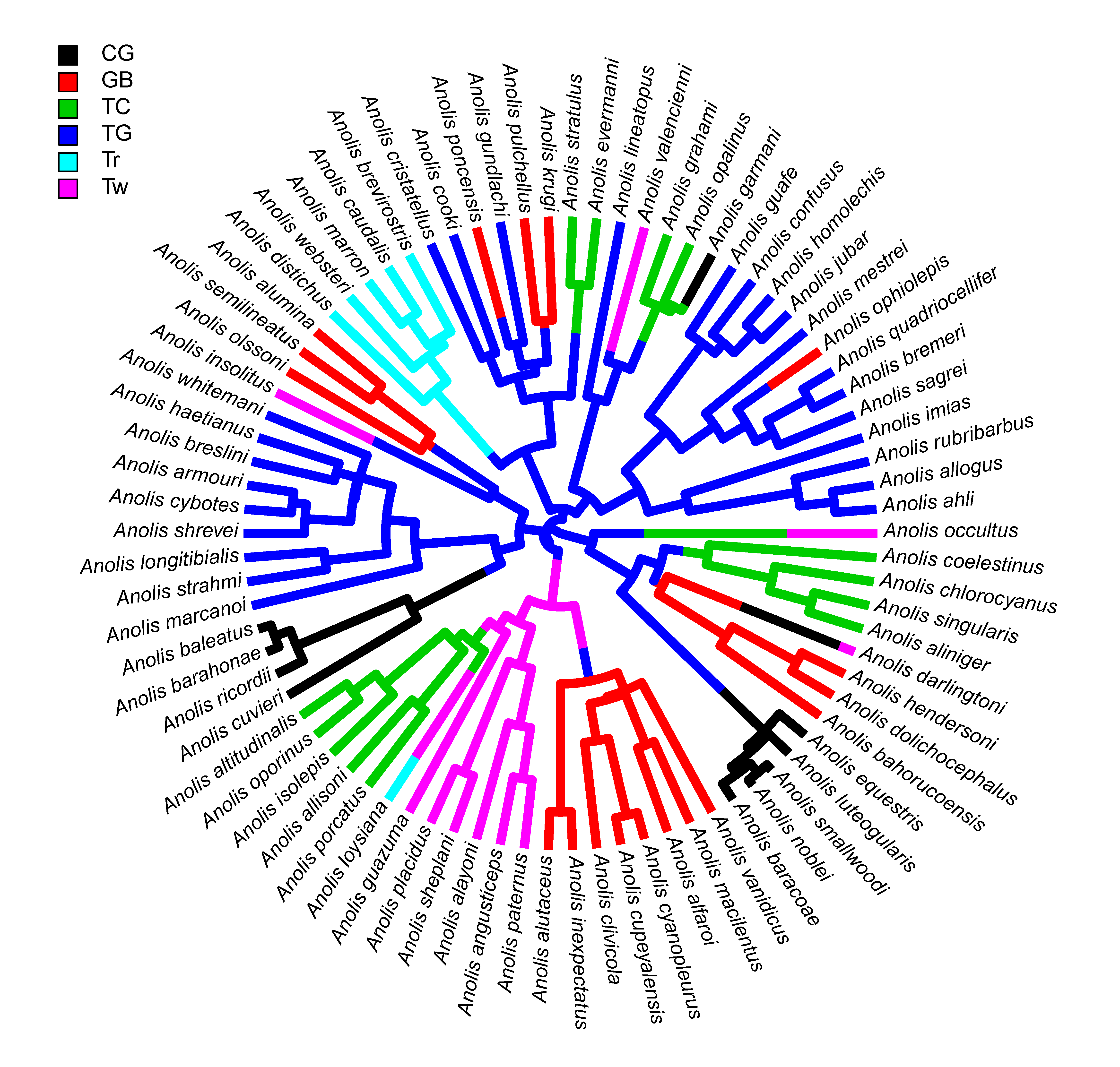
plot(anoletree,lwd=5,ftype="i",fsize=0.5)

## no colors provided. using the following legend:
##        CG        GB        TC        TG        Tr        Tw 
##   "black"     "red"  "green3"    "blue"    "cyan" "magenta"

plot(anoletree,lwd=5,ftype="i",fsize=0.5,lend=0) ## curved

## no colors provided. using the following legend:
##        CG        GB        TC        TG        Tr        Tw 
##   "black"     "red"  "green3"    "blue"    "cyan" "magenta"

plot(anoletree,lwd=5,ftype="i",fsize=0.5,lend=1) ## mitered

## no colors provided. using the following legend:
##        CG        GB        TC        TG        Tr        Tw 
##   "black"     "red"  "green3"    "blue"    "cyan" "magenta"

Or as type="fan"

plot(anoletree,lwd=5,ftype="i",fsize=0.8,lend=1,type="fan")

## no colors provided. using the following legend:
##        CG        GB        TC        TG        Tr        Tw 
##   "black"     "red"  "green3"    "blue"    "cyan" "magenta"

cols<-setNames(palette()[1:length(unique(getStates(anoletree,
"tips")))],
    sort(unique(getStates(anoletree,"tips"))))
add.simmap.legend(colors=cols,x=0.9*par()$usr[1],
    y=0.9*par()$usr[4],prompt=FALSE,fsize=0.9)

Note that the 'pixelation' (aka. aliasing) is just an effect of the rendering and disappears if the plot is rendered as a PDF, e.g.:

Finally, the purpose of plotting the two lines originating at the root as a single segmented line is the eliminate what can be an ugly overlap of the two daughter edges when plotted separately:

plotTree(tree,type="fan",lwd=4,part=0.5,lend=1,fsize=0.5)

or:

(rendered more nicely).

That's it.

I just pushed a series of updates (1, 2, 3, 4) to fix some issues raised by the authors of ape and phangorn in advance of the submission of new CRAN versions of those two packages.

The first was that I had inadvertently corrupted an S3 method multi2di of ape when I created the function multi2di.simmap without exporting a method to the namespace. The other issues came up in R CMD check and included such things as failing to import various functions from dependencies, other problems with the namespace, errors in documenting various variables, the absence of a manual page for one function (likSurface.rateshift) that is exported by phytools, and a few problems with the R code of some new functions.

I too hope to update the version of phytools on CRAN as the current version dates to June.

The latest phytools version can be installed from GitHub using devtools as follows:

library(devtools)
install_github("liamrevell/phytools")

Since both phangorn & ape are in the process of being updated, but phytools depends on the latest version of neither, you may need to do:

install_github("liamrevell/phytools",upgrade_dependencies=FALSE)

That's it.

In advance of a workshopI'll be teaching next week at the Universidad Nacional del Comahue in (reputedly) beautiful Bariloche, Argentina, I will be trying to get a new version of phytools on CRAN. This update will have version number >=0.5.62 (TBD).

It has been over five months since I last submitted a phytools update to CRAN. Obviously, there have been a ton of updates in that time. Here are some:

1. A bug fix in collapseTree.
2. More user control of the plot method for phylo.toBackbone (here).
3. Another updateto backbonePhylo to permit multiple clades to have the same label.
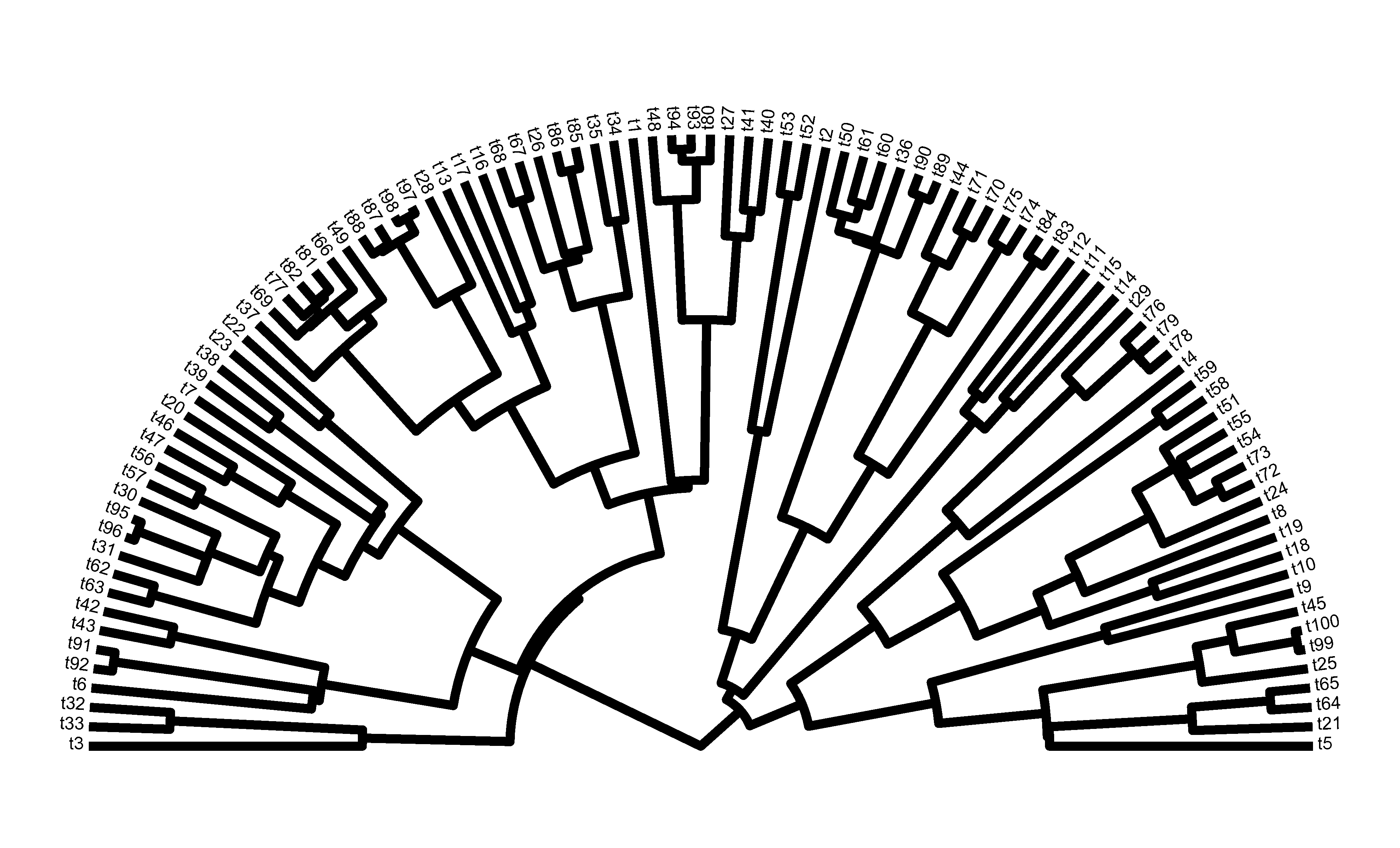
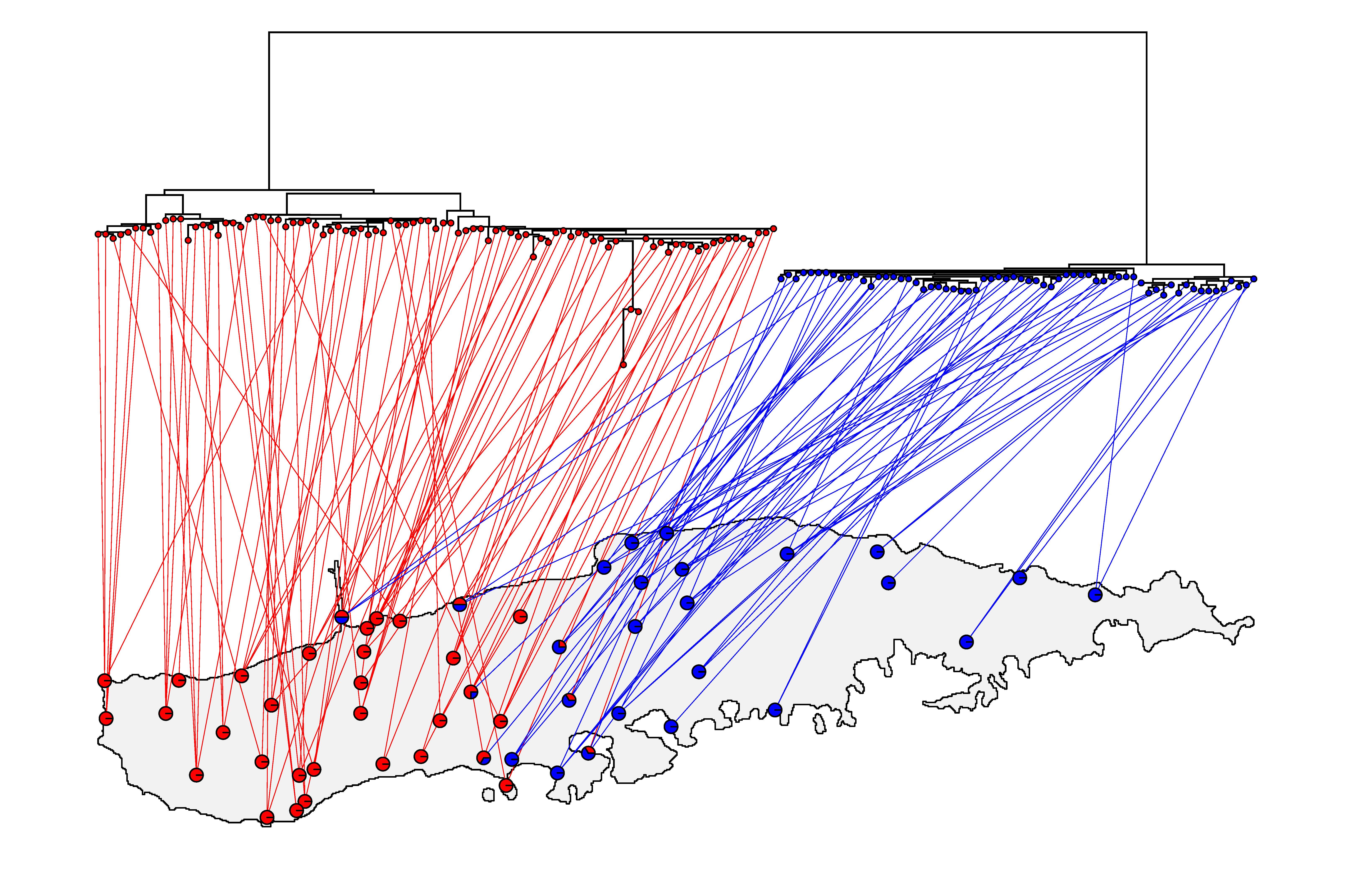
4. Various updatesto phylo.to.map which helped enable this nice plot:
5. A new phytools function for showing a barplot next to a plotted tree, plotTree.barplot (1, 2, 3).
6. A new function, related to plotTree.barplot, to plot a boxplot next to a phylogeny (plotTree.boxplot). Also see this additionpermitting the boxplot to be build using the ‘formula’ method.
7. A simple updateto phyl.pca to permit more columns than rows in the input data matrix.
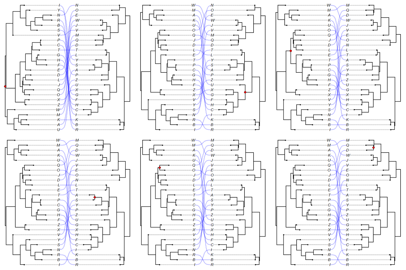
8. Updateto plot.cophylo to permit sigmoidal linking lines.
9. New functionto resolve a polytomous node in all possible ways. (Also here.)
10. Function to reorder the daughter edges of a multifurcation in all possible ways.
11. New option to rotate polytomies for co-phylogenetic plotting using the algorithm developed for [10.] (here).
12. Speed up & fixes for collapseTree.
13. New option to get the variance and confidence intervals for reconstructed tip states obtained using anc.ML.
14. New function to plot the likelihood surface for the phytools function rateshift.
15. Update to the function add.color.barto permit the gradient color legend to be plotted vertically as well as horizontally.
16. Additional user control of the S3 plot method for objects of class "cophylo".
17. Updates to tip label plotting and a new S3 summarymethod for "cophylo" class objects.
18. A newphytools function to find all possible node rotations of all nodes in a tree.
19. A new exhaustive search for the cophylo function for co-phylogenetic plotting.
20. Some updates to fitMkto permit more user control of optimization.
21. A small fixto pass optional arguments to fitMk within make.simmap.
22. A fun animated optimization method for cophylo. The animation, shown below, shows the tree traversal and the node rotations of the tree gradually being improved by the algorithm:
23. A bug fix for add.color.bar.
24. A very simple new cospeciationtest in phytools.
25. A function to compute a modifiedversion of Grafen’s edge lengths.
26. A cool S3 densitymethodfor objects of class "multiSimmap".
27. Some new methodsand user-control of phylogenetic scattergram plotting using fancyTree.
28. Some updatesto permit more user control of line end types in plotSimmap.
29. An extremely simplefunction (bd) to pull birth & death (species & extinction) rates from an object of class "birthdeath" computed by ape.
30. A simple new functionand printmethod to compute AIC weights.
31. And, finally, a bunch of other miscellaneousupdates to address issues raised when updating ape & phangorn.

I know this isn't comprehensive, but it is a survey reflecting the wide range of updates & changes to the package. Of course, now that phytools is on GitHub, it's super easy to track all the committedchanges the package has seen.

I'll post again when the updated phytools makes it on CRAN!

phytools 0.5-64 is now available from CRAN.

install.packages("phytools",repos="https://cloud.r-project.org")

## Installing package into 'C:/../R/win-library/3.3'
## (as 'lib' is unspecified)

## package 'phytools' successfully unpacked and MD5 sums checked

packageVersion("phytools")

## [1] '0.5.64'

[As of about 7am, December 6 it looks like Windows binaries have been built, but not binaries for Mac OS. Consequently, Mac users may want to hold off updating or install from source. Installing phytools from source is super-easy as phytools does not require compilation. Just add the argument type="source" to install.packages&voila!]

I recently received the following user request:

“I have a small question regarding your phytools function plotBranchbyTrait that I was hoping you perhaps could help with. I am trying to visualize [my data with range 0 to 1] using the heat.color palette. However, as some species have a proportion of 0, and others have a proportion of 1, the branches leading to the latter are almost white and thus impossible to see. If I change the proportion of one of these species to, say 1.2, most of branches become more visible (except the branch leading to that particular species of course). However, this is not an ideal way to go about it. Is there any way I can make sure to only use parts of the color palette for the plot, excluding the brightest, white colors?”

Indeed, this effect can easily be verified using simulation:

library(phytools)
tree<-pbtree(n=100)
x<-fastBM(tree,scale=1)
plotBranchbyTrait(tree,x,"tips","heat.colors",show.tip.label=FALSE)

We can see that tips & edges with the most extreme values of the trait essentially vanish.

[Note that plotBranchbyTrait is unusual among phytools functions in that it uses ape::plot.phylo internally instead of plotSimmap in my package - hence the argument show.tip.label=FALSE which would be ftype="off"in most other phytools functions.]

The easiest way to address this was to allow the argument paletteto be supplied as a function as well as as a string. I pushed this update to GitHub already & it can be seen here.

Here's an example:

plotBranchbyTrait(tree,x,"tips",
    palette=colorRampPalette(c("red","orange","yellow")),
    show.tip.label=FALSE)

We can even write our own custom function, for instance using the original heat.colors palette function internally, but cutting off the last (say) 5% of the spectrum:

foo<-function(n){
    obj<-heat.colors(round(1.05*n))
    obj[1:n]
}
plotBranchbyTrait(tree,x,"tips",palette=foo,show.tip.label=FALSE)

Finally, because plotBranchbyTrait uses plot.phylointernally, we can use any of the plot.phylo options, such as:

plotBranchbyTrait(tree,x,"tips",foo,type="fan",show.tip.label=FALSE,
    legend=1.8)

plotBranchbyTrait(tree,x,"tips",foo,type="unrooted",show.tip.label=FALSE,
    legend=1.8)

and so on.

To get this update you can install phytools from GitHub using the package 'devtools' as follows:

library(devtools)
install_github("liamrevell/phytools")

I was just corresponding with a phytools user & essentially the lack of an argument node.col in the function phylomorphospace3d was broached.

Why this option doesn't exist, I couldn't tell you; however it is relatively easy to circumvent because the function invisibly returns a list of functions which can be used to plot points, lines, planes, etc., back in the original (simulated) space.

Here's a quick example, using simulated data:

library(phytools)
tree ## our tree

## 
## Phylogenetic tree with 26 tips and 25 internal nodes.
## 
## Tip labels:
##  A, B, C, D, E, F, ...
## 
## Rooted; includes branch lengths.

X ## our data

##          [,1]         [,2]        [,3]
## A -2.84172235  1.148037248  1.64782403
## B -2.05052328  1.431708869  1.15202298
## C -1.24686168  1.946696167  1.54897262
## D -0.52310503  0.573110584  0.46436125
## E -0.55578283  0.813448906  0.40254794
## F -0.51150759  1.733066759  1.49429840
## G  0.53936198  1.816801753  1.86050506
## H  0.01234429  2.302339855  2.63078614
## I -0.01684737  1.810997083  2.22857705
## J  1.32317051  2.492348110  0.55660832
## K  0.39032083  1.138053408 -0.42215854
## L  1.35224610  0.701773929 -0.73233992
## M  0.06642055  2.393143196  1.67769111
## N  0.53170462  2.387858206  1.07395647
## O  1.33893651  1.869361233  1.18002858
## P  0.16788769  1.722551818  0.03908209
## Q  0.72826260  0.591128118  1.23662094
## R  0.79698877  1.310841641  1.38182879
## S  0.08976056  1.727227579  2.10565084
## T  1.37506375 -0.551729936 -1.73123720
## U -1.09244120  0.960226117 -1.01694632
## V -0.75692309 -0.002878853 -1.02230472
## W -0.53535698 -0.168545803 -1.33846396
## X -0.26869690 -0.241183840 -1.14188545
## Y  0.19315024  0.282576551 -0.89620379
## Z -0.56460363 -0.613852876  0.98093216

y ## our character we want to map on the tips

##   A   B   C   D   E   F   G   H   I   J   K   L   M   N   O   P   Q   R 
## "c" "c" "b" "b" "b" "a" "a" "b" "b" "c" "c" "b" "c" "c" "c" "a" "c" "b" 
##   S   T   U   V   W   X   Y   Z 
## "b" "b" "c" "b" "c" "c" "c" "c"

tip.col<-y
tip.col[tip.col=="a"]<-"red"
tip.col[tip.col=="b"]<-"blue"
tip.col[tip.col=="c"]<-"yellow"
obj<-phylomorphospace3d(tree,X,method="static")
obj$points3d(X,cex=1.4,pch=21,bg=tip.col[rownames(X)])

That's it.

The tree & data were simulated as follows:

X<-fastBM(tree,nsim=3)
Q<-matrix(c(-1,1,0,1,-2,1,0,1,-1),3,3)
rownames(Q)<-colnames(Q)<-c("a","b","c")
y<-sim.history(tree,Q)$states

I just got back from teaching a five-day workshop the Universidad Nacional del Comahue in San Carlos de Bariloche, Argentina.

It was tiring, but a lot of fun - and I hope it was as rewarding for the students as it was for me.

As has become a tradition in the Latin American workshops that I teach (e.g., 1, 2, 3, 4, etc.), we have a course t-shirt - and, not only that, the t-shirt must be designed in R.

This year's workshop in Bariloche was not spared. Firstly, the design:

library(phytools)

## Loading required package: ape

## Loading required package: maps

library(plotrix)
source("http://www.phytools.org/Bariloche2016/data/arctext.R")
set.seed(545)
tree<-pbtree(n=78,scale=0.8)
txt<-write.tree(tree)
txt<-strsplit(txt,";")[[1]]
txt<-paste("((Y:0.9,",txt,":0.1):0.1,Z:1);",sep="")
tree<-read.tree(text=txt)
tree<-phytools:::lambdaTree(tree,0.95)
tree<-make.era.map(tree,c(0,0.4,0.8))
par(bg="darkgrey")
par(ljoin=1,lmitre=30)
par(mar=rep(0,4))
col<-rgb(red=117/255,green=170/255,blue=219/255)
par(fg="transparent")
plot(tree,colors=setNames(rep("black",3),1:3),
    lwd=10,type="fan",part=0.5,ftype="off",ylim=c(-0.2,1.2),
    lend=1)
par(fg="black")
plot(tree,colors=setNames(c(col,"white",col),1:3),
    lwd=8,type="fan",part=0.5,ftype="off",ylim=c(-0.2,1.2),
    lend=1,add=TRUE)
text(mean(par()$usr[1:2]),-0.15,"Bariloche, Argentina 2016",
    col="black",cex=2.7,font=2)
chars<-strsplit("Latin American Macroevolution Workshop","")[[1]]
stretch<-rep(1.1,length(chars))
arctext("Latin American Macroevolution Workshop",center=c(0,0),radius=1.1,
    cex=3.5,font=2,stretch=stretch)

(High resolution PDF with Times font for the text here.)

The only small wrinkle is that I tweaked the code of arctext in the plotrix package to get the text to look the way I wanted it to.

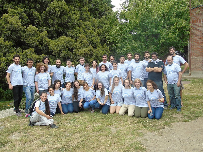
Finally, but most importantly, the students (& me) sporting our t-shirts:

(Click on image for larger version.)

Many thanks to course organizers Lina Moreno Azócar& Félix Cruz, who were wonderful hosts, helped put together a terrific course, and who also had the wonderful patience to drive me back & forth across the border to Chile (no small task) so I didn't have to fly through Buenos Aires!

Until next time Argentina!

A phytools user asks the following:

“I am following your blog. I have a phylogenetic tree. I would like to color the tree according to their genus name. Could you please help me, providing the code in R?”

There are in fact many ways to plot a tree with edges or clades in different colors. I'm going to give a demo using paintSubTree and plotSimmap in phytools as follows.

First, let's imagine the following species-level tree in which I have used the syntax Genus_species for all taxon labels.

library(phytools)
species.tree

## 
## Phylogenetic tree with 56 tips and 55 internal nodes.
## 
## Tip labels:
##  Rfom_nhijvq, Nvztxu_evipjo, Bswlbtch_azndgw, Ghsygvn_azkqlr, Qptbc_lwcqya, Qptbc_tpnozk, ...
## 
## Rooted; includes branch lengths.

plotTree(species.tree,ftype="i",fsize=0.7,color="black")

First, let's identify all the genera:

genera<-sapply(species.tree$tip.label,function(x) strsplit(x,"_")[[1]][1])
genera<-sort(unique(genera))
genera

##  [1] "Bswlbtch" "Dxfnqt"   "Fyoed"    "Gdzxskm"  "Ghsygvn"  "Nvztxu"  
##  [7] "Pxvolmfp" "Qpebj"    "Qptbc"    "Rfom"     "Sehvikuc" "Sfownt"  
## [13] "Uspvk"    "Uvybs"    "Wpuqdc"   "Wqbhd"

Next, find the MRCA of each genus. In the event that the genus contains only one member, we can just paint the terminal edge:

for(i in 1:length(genera)){
    ii<-grep(genera[i],species.tree$tip.label)
    ca<-if(length(ii)>1) 
        findMRCA(species.tree,species.tree$tip.label[ii]) else ii
    species.tree<-paintSubTree(species.tree,ca,state=as.character(i),
        anc.state="0",stem=TRUE)
}

The following is a trick to remove map segments of zero length:

tol<-max(nodeHeights(species.tree))*1e-12
species.tree$maps<-lapply(species.tree$maps, function(x,tol) 
    if(length(x)>1) x[-which(x<tol)] else x,tol=tol)

Now we can set our colors & plot them:

cols<-setNames(c("grey",rainbow(length(genera))),
    0:length(genera))
plot(species.tree,fsize=0.7,colors=cols,ftype="i",split.vertical=TRUE,
    lwd=3,xlim=c(-24,120))
par(font=3)
add.simmap.legend(colors=setNames(cols[2:length(cols)],genera),fsize=0.8,
    prompt=FALSE,x=-24,y=24)

That's basically the idea.

The tree for this example is obviously simulated. The following is the code that was used for simulation (taken from a previous post, here)::

library(phytools)
## first let's simulate our genus tree:
foo<-function() paste(sample(LETTERS,1),paste(sample(letters,
    round(runif(1,min=3,max=7))),collapse=""),sep="")
genera<-replicate(16,foo())
genus.tree<-pbtree(n=length(genera),tip.label=genera,scale=80)
genus.tree$edge.length[which(genus.tree$edge[,2]<=Ntip(genus.tree))]<-
    genus.tree$edge.length[which(genus.tree$edge[,2]<=Ntip(genus.tree))]+20
tips<-c()
for(i in 1:Ntip(genus.tree)){
    n.genus<-sample(1:6,1)
    if(n.genus>0) for(j in 1:n.genus) 
        tips<-c(tips,paste(genus.tree$tip.label[i],
        paste(sample(letters,6),collapse=""),sep="_"))
}
## add them:
species.tree<-genus.to.species.tree(genus.tree,tips)

I just addeda tiny update to phytools in which I have included a new S3 method to convert an object of class "phylo" to an object of class "multiPhylo".

This is super-simple & looks something like the following:

as.multiPhylo.phylo<-function(x,...){
    obj<-list(x)
    class(obj)<-"multiPhylo"
    obj
}

as.multiPhylo<-function(x,...){
    if (identical(class(x),"multiPhylo")) return(x)
    UseMethod("as.multiPhylo")
}

(along with appropriate S3method declaration in NAMESPACE, etc.).

The purpose of this is to allow a function to return an object of a consistent class, even if it sometimes returns only one tree. This might be for example, read.nexus (in which our input files may contain only 1 phylogeny), or pbtree, in which a variable number of phylogenies are to be simulated.

Here is a quick demo of the latter:

pbtree(n=26,tip.label=LETTERS)

## 
## Phylogenetic tree with 26 tips and 25 internal nodes.
## 
## Tip labels:
##  A, B, C, D, E, F, ...
## 
## Rooted; includes branch lengths.

pbtree(n=26,tip.label=LETTERS,nsim=10)

## 10 phylogenetic trees

vs.

as.multiPhylo(pbtree(n=26,tip.label=LETTERS))

## 1 phylogenetic trees

as.multiPhylo(pbtree(n=26,tip.label=LETTERS,nsim=10))

## 10 phylogenetic trees

The update can be obtained by installing phytools version >= 0.5-67 from GitHub.

I just added S3 print, residuals, and coef methods for the phylogenetic reduced major axis regression function, phyl.RMA. The updates can be seen here.

The following is a quick demo using simulated data:

library(phytools)
packageVersion("phytools")

## [1] '0.5.68'

tree

## 
## Phylogenetic tree with 26 tips and 25 internal nodes.
## 
## Tip labels:
##  A, B, C, D, E, F, ...
## 
## Rooted; includes branch lengths.

x

##           A           B           C           D           E           F 
##  5.02625173  3.84069323  1.40907359  1.62584177 -0.38820852 -0.03660051 
##           G           H           I           J           K           L 
## -1.15405529 -1.05555766 -1.10500369 -1.82982215 -0.58220778 -0.62621299 
##           M           N           O           P           Q           R 
##  2.58984857  1.65864863  1.38732527  1.10492094  0.89527230 -1.40154533 
##           S           T           U           V           W           X 
##  1.23500803 -0.24029572 -0.26507837 -0.77611134 -0.88118355 -2.59262521 
##           Y           Z 
## -0.11687224 -1.68772212

y

##           A           B           C           D           E           F 
##  5.03364484  4.45525372  2.33034028  1.70260435  1.86376515  0.63005315 
##           G           H           I           J           K           L 
## -1.27847189 -0.51986100  0.42627759 -0.59603022 -1.02732412 -1.06377260 
##           M           N           O           P           Q           R 
##  0.11285994  0.08066473 -0.02928941 -0.14296226 -0.38034287 -2.11329071 
##           S           T           U           V           W           X 
## -0.12823996  1.88409506  2.23634682 -0.82779628 -0.49460318 -2.37103424 
##           Y           Z 
## -2.07654579 -0.58623675

phylomorphospace(tree,cbind(x,y),node.size=c(0,0))
points(cbind(x,y),cex=1.2,pch=21,bg="grey")

Now let's run the RMA regression:

obj<-phyl.RMA(x,y,tree)
## print
obj

## 
## Coefficients:
## (Intercept)           x 
##  -0.0424625   1.0647447 
## 
## VCV matrix:
##          x        y
## x 1.504905 1.119709
## y 1.119709 1.706083
## 
## Model for the covariance structure of the error is "BM"
## 
## Estimates (or set values):
##    lambda    log(L) 
##   1.00000 -69.49404 
## 
## Hypothesis test based on Clarke (1980; Biometrika):
##        r2         T        df         P 
##  0.488316  0.429650 21.290154  0.671767 
## 
## Note that the null hypothesis test is h0 = 1

coef(obj)

## (Intercept)           x 
##  -0.0424625   1.0647447

residuals(obj)

##            A            B            C            D            E 
## -0.275567308  0.408358649  0.872499213  0.013960519  2.319570602 
##            F            G            H            I            J 
##  0.711485847 -0.007235186  0.646500875  1.645286860  1.394725642 
##            K            L            M            N            O 
## -0.364958989 -0.354553159 -2.602204971 -1.642910026 -1.463974066 
##            P            Q            R            S            T 
## -1.276958414 -1.291116753 -0.578540317 -1.400745657  2.182411146 
##            U            V            W            X            Y 
##  2.561050105  0.041026621  0.486094798  0.431912090 -1.909644200 
##            Z 
##  1.253218854

I also wrote a simple plot method that throws the RMA line on top of a plotted phylomorphospace. Details can be seen here.

This is what it looks like:

plot(obj)

We can also flip x or y just to see what it looks like to plot a negative slope. Note that we can only test a null hypothesis that has the same sign as our fitted RMA line. Here (for fun), I'll test the null hypothesis h₀ = -2/3.

neg.x<--x
obj<-phyl.RMA(neg.x,y,tree,h0=-2/3)
obj

## 
## Coefficients:
## (Intercept)           x 
##  -0.0424625  -1.0647447 
## 
## VCV matrix:
##           x         y
## x  1.504905 -1.119709
## y -1.119709  1.706083
## 
## Model for the covariance structure of the error is "BM"
## 
## Estimates (or set values):
##    lambda    log(L) 
##   1.00000 -69.49404 
## 
## Hypothesis test based on Clarke (1980; Biometrika):
##        r2         T        df         P 
##  0.488316  3.206537 21.290154  0.004187 
## 
## Note that the null hypothesis test is h0 = -0.666666666666667

plot(obj)

That's the idea anyway.

Data for this demo were simulated as follows:

library(phytools)
tree<-pbtree(n=26,tip.label=LETTERS)
xy<-fastBM(tree)
x<-xy+fastBM(tree,sig2=0.4)
y<-xy+fastBM(tree,sig2=0.4)

A phytools user contacted me the other day about getting reconstructed internal values instead of at nodes, at different time slices of the tree.

His idea was to extract these from a "contMap" object, but since contMap is primarily for visualization (and finally discretizes time), a more sensible approach is to simply re-root the tree at each of the desired time slices and compute the values for those slices.

Note that now our values will correspond to points along edges, rather than to number internal nodes.

Here, I'll demo this using a tree with 26 taxa & total depth of 100, sampling edge states at depths 25, 50, & 75 - but roughly the same procedure should work on any tree.

First, here are our data:

library(phytools)
tree

## 
## Phylogenetic tree with 26 tips and 25 internal nodes.
## 
## Tip labels:
##  A, B, C, D, E, F, ...
## 
## Rooted; includes branch lengths.

x

##           A           B           C           D           E           F 
##  -5.8903745  -5.7282584   0.5445433 -13.8386694 -14.0666611  -5.6192333 
##           G           H           I           J           K           L 
##   0.2928983  -8.9493757  -9.2341163 -13.2477565 -18.3027044 -20.3522182 
##           M           N           O           P           Q           R 
## -22.4985786 -25.7573926  -6.8546698  -9.4871527 -17.8719246  13.8470125 
##           S           T           U           V           W           X 
##  17.0261569  11.0099036   8.9560054  19.7438105  10.0868538   8.2936089 
##           Y           Z 
##   3.1156954   3.5875638

plotTree(tree,mar=c(4.1,1.1,1.1,1.1))
axis(1)
abline(v=c(25,50,75),lty="dashed")
nodelabels()

Note that for each time slice, obviously we are going to get different numbers of states (3, 9, & 13 in this case).

Now, let's do it for time slice t = 25:

H<-nodeHeights(tree)
t<-25
ii<-intersect(which(H[,1]<=t),which(H[,2]>t))
node<-tree$edge[ii,2]
position<-t-H[ii,1]
rerooted<-mapply(reroot,node=node,position=position,
    MoreArgs=list(tree=tree),SIMPLIFY=FALSE)
foo<-function(ind,tree) paste(tree$edge[ind,],collapse=",")
a25<-setNames(sapply(rerooted,function(t,x) fastAnc(t,x)[1],x=x),
    sapply(ii,foo,tree=tree))
a25

##     28,29     28,34     27,44 
## -4.797286 -7.056366  4.821428

As you can see, I've set the names of a25 to match the starting & ending node indices as plotted above.

We can of course repeat the same procedure for each of our time slices:

## time 50
t<-50
ii<-intersect(which(H[,1]<=t),which(H[,2]>t))
node<-tree$edge[ii,2]
position<-t-H[ii,1]
rerooted<-mapply(reroot,node=node,position=position,
    MoreArgs=list(tree=tree),SIMPLIFY=FALSE)
foo<-function(ind,tree) paste(tree$edge[ind,],collapse=",")
a50<-setNames(sapply(rerooted,function(t,x) fastAnc(t,x)[1],x=x),
    sapply(ii,foo,tree=tree))
a50

##      30,31      30,32       29,6      34,35      38,39      38,42 
##  -5.685643  -5.788953  -5.558655  -9.855100 -12.692816 -11.479507 
##      44,45      46,47      46,51 
##   8.854554   7.781511   7.332690

## time 75
t<-75
ii<-intersect(which(H[,1]<=t),which(H[,2]>t))
node<-tree$edge[ii,2]
position<-t-H[ii,1]
rerooted<-mapply(reroot,node=node,position=position,
    MoreArgs=list(tree=tree),SIMPLIFY=FALSE)
foo<-function(ind,tree) paste(tree$edge[ind,],collapse=",")
a75<-setNames(sapply(rerooted,function(t,x) fastAnc(t,x)[1],x=x),
    sapply(ii,foo,tree=tree))
a75

##      30,31      30,32       29,6       37,7       37,8       36,9 
##  -5.748358  -6.702843  -5.588944  -6.015129  -8.228368  -8.797681 
##      35,10      38,39      42,43      42,17      44,45      47,48 
## -10.128888 -18.896693 -11.157098 -13.541521  12.638761   9.604015 
##      47,49      46,51 
##  12.091764   5.072981

If we overlay these points on a 'traitgram' style visualization, we should see that they fall directly on the lines of our plot.

phenogram(tree,x,spread.cost=c(1,0))
abline(v=c(25,50,75),lty="dashed")
points(rep(25,length(a25)),a25,pch=21,bg="grey",cex=1.2)
points(rep(50,length(a50)),a50,pch=21,bg="grey",cex=1.2)
points(rep(75,length(a75)),a75,pch=21,bg="grey",cex=1.2)

You get the idea. Cool!

I recently received the following request:

“I would love to know if there is any way of extracting and colouring only a certain set of the terminal edges of the phylogeny, based on the tip labels. For example, using edge.color within plot.phylo based on a vector of tips. Do you know of any code that could be used to do this.”

This is pretty straightforward to do using phytools. Note that it can also be done using plot.phylo in the ape package, but I'm going to focus on the phytools way for obvious reasons.

I'll image that I'm painting the terminal edges leading to each tip with different colors based on the state of a discrete trait - but we could modify our technique for any arbitrary grouping of tips.

Here's the tree & data:

library(phytools)
tree

## 
## Phylogenetic tree with 26 tips and 25 internal nodes.
## 
## Tip labels:
##  A, B, C, D, E, F, ...
## 
## Rooted; includes branch lengths.

x

## A B C D E F G H I J K L M N O P Q R S T U V W X Y Z 
## c a c a a c c a a a b c c a c b a a b c c b c a a b 
## Levels: a b c

Now, let's say we want to color the edges blue & red respectively if the corresponding edge is in state b or c, respectively, and leave it black if the tip is in state a.

## identify the tips in states b or c
b<-names(x)[x=="b"]
b

## [1] "K" "P" "S" "V" "Z"

c<-names(x)[x=="c"]
c

##  [1] "A" "C" "F" "G" "L" "M" "O" "T" "U" "W"

## paint the edges
tt<-paintBranches(tree,edge=sapply(b,match,tree$tip.label),
    state="b",anc.state="a")
tt<-paintBranches(tt,edge=sapply(c,match,tree$tip.label),
    state="c")

Now we can plot our tree:

tt

## 
## Phylogenetic tree with 26 tips and 25 internal nodes.
## 
## Tip labels:
##  A, B, C, D, E, F, ...
## 
## The tree includes a mapped, 3-state discrete character with states:
##  a, b, c
## 
## Rooted; includes branch lengths.

cols<-setNames(c("black","blue","red"),c("a","b","c"))
plot(tt,colors=cols,lwd=4,split.vertical=TRUE,ftype="i")

Let's check this against a plot generated using dotTree:

dotTree(tree,x,colors=cols)

That's about it.

Tree & data for this demo were simulated as follows:

tree<-pbtree(n=26,tip.label=LETTERS)
Q<-matrix(c(-2,1,1,1,-2,1,1,1,-2),3,3)
rownames(Q)<-colnames(Q)<-letters[1:3]
x<-as.factor(sim.history(tree,Q)$states)

A phytools user recently posted the following question:

“Is there a blog post / function capable of combining the functionality of contmap and dottree? I'm looking to plot a continuous character with a color ramp on the tree with a discrete character dot next to the tips of the tree. If I there is a post on this I have missed it in my search and would appreciate being pointed in the right direction if it is out there.”

The answer is that this is pretty straightforward to do - though it does take a little investigating of the internals of each function.

Here my approach will be to compute a "contMap" object & then overlay it on top of a plotted dotTree.

We can start by imagining the following data:

library(phytools)
tree

## 
## Phylogenetic tree with 26 tips and 25 internal nodes.
## 
## Tip labels:
##  A, B, C, D, E, F, ...
## 
## Rooted; includes branch lengths.

x

## A B C D E F G H I J K L M N O P Q R S T U V W X Y Z 
## c c c b a c c c c c c b a a b b b b b c c c b a a a 
## Levels: a b c

y

##       A       B       C       D       E       F       G       H       I 
## -0.7592 -0.9114 -1.1249  0.0006 -0.8630  2.5855  2.8233  2.4789  2.3854 
##       J       K       L       M       N       O       P       Q       R 
## -2.5600 -2.3400 -2.3566 -1.8551 -1.6360 -0.4659 -3.1787 -2.8704 -0.0257 
##       S       T       U       V       W       X       Y       Z 
##  0.3514  0.0436  0.9419 -0.2918 -0.6332 -0.5828 -0.3969 -2.1122

Next, we compute our "contMap" object, but we don't plot it:

obj<-contMap(tree,y,plot=FALSE)
obj

## Object of class "contMap" containing:
## 
## (1) A phylogenetic tree with 26 tips and 25 internal nodes.
## 
## (2) A mapped continuous trait on the range (-3.1787, 2.8233).

Finally, we plot our discrete character using dotTree after which we overlay our contMap style plot. This is the tricky part because I had to look up & duplicate the internal plotting parameters of dotTree to ensure that the two trees where directly overlain:

cols<-setNames(c("black","red","blue"),c("a","b","c"))
dotTree(tree,x,colors=cols,lwd=7)
par(fg="transparent")
plot(obj$tree,add=TRUE,lwd=5,colors=obj$cols,
    ylim=c(-1/25*Ntip(tree),Ntip(tree)),offset=1.7)
par(fg="black")
add.color.bar(0.3*max(nodeHeights(tree)),obj$cols,title="trait value",
    lims=obj$lims,digits=3,prompt=FALSE,x=0.3*max(nodeHeights(tree)),
    y=0.4*(1+par()$usr[3]),lwd=4,fsize=1,subtitle="")

That's it!

In response to a user comment I have added a feature to plotTree.barplot to permit multiple traits or values to be plotted for each species - either using stacked bars, or by plotting the bars side-by-side.

The update can be seen here. The problem turned out to be a little bit mroe complicated then it seemed it first, mainly because of a quirk in barplot that means that the object returned by boxplot (which I then use to correctly space the tips of the plotted tree) differs depending on whether the input data come in the form of a vector of single values or a matrix, &, if the latter, whether the argument beside=TRUE is selected or not.

Here's a quick & dirty demo. These data are (simulated to represent) relative frequencies - said dietary fraction of three different food types - so stacking of our bars is appropriate:

library(phytools)
packageVersion("phytools")

## [1] '0.5.70'

tree

## 
## Phylogenetic tree with 26 tips and 25 internal nodes.
## 
## Tip labels:
##  A, B, C, D, E, F, ...
## 
## Rooted; includes branch lengths.

X

##        plant  vertebrate invertebrate
## A 0.31086049 0.212175943   0.47696356
## B 0.15404215 0.440976975   0.40498087
## C 0.26982034 0.450834511   0.27934515
## D 0.12260206 0.358475976   0.51892197
## E 0.29979068 0.129743168   0.57046615
## F 0.20163877 0.440001107   0.35836012
## G 0.05465514 0.410528162   0.53481670
## H 0.47392116 0.121520364   0.40455848
## I 0.44344594 0.101251541   0.45530252
## J 0.24839375 0.268691107   0.48291514
## K 0.12309160 0.101699889   0.77520851
## L 0.24010676 0.065417274   0.69447597
## M 0.23424489 0.226431850   0.53932326
## N 0.40030662 0.057542453   0.54215092
## O 0.15332681 0.023255378   0.82341781
## P 0.44389924 0.491496743   0.06460401
## Q 0.27010640 0.292077796   0.43781581
## R 0.21643656 0.208244073   0.57531937
## S 0.19650159 0.317376110   0.48612230
## T 0.01261411 0.427646672   0.55973922
## U 0.32707264 0.164682573   0.50824478
## V 0.28931830 0.126987763   0.58369394
## W 0.08407750 0.252999348   0.66292315
## X 0.28631262 0.004105909   0.70958147
## Y 0.38118921 0.206806916   0.41200387
## Z 0.07941718 0.074216139   0.84636668

plotTree.barplot(tree,X)

Or, we can plot the bars side-by-side:

plotTree.barplot(tree,X,args.barplot=list(beside=TRUE,xlim=c(0,1),
    legend.text=TRUE,space=c(0,1.2),args.legend=list(x=1,y=17)))

Note that beside=FALSE is not a good option if our data have both positive & negative values as this can produce a weird result. For instance:

Y

##         [,1]        [,2]        [,3]
## A  0.7618018  2.59661203 -0.23590050
## B  0.8548063  1.40920654  0.73019040
## C -1.1970456  1.09259205  0.56974523
## D -0.4355176  2.31904920 -1.18347277
## E  2.2923226  2.35986558 -3.22201293
## F  2.5004466  3.98754763 -2.68168275
## G  2.7103706  1.94742983 -1.81626643
## H  1.4677625  1.90001387 -2.78720751
## I  1.5596683  4.57540030 -0.17596327
## J  1.5259543  5.22197986 -0.50073032
## K  1.4834068  4.99761663 -0.35070911
## L  1.3819468  4.84211948 -0.49581275
## M  1.4874512  4.99309837 -0.06583491
## N  0.3560632  3.50340705 -0.95027035
## O -0.2002478  3.80948866 -0.60808238
## P -0.9702761  3.93130784 -3.55745209
## Q -0.2638056  2.81862255 -2.47669725
## R  0.6922559  3.11378711 -3.53855007
## S -0.5630365  3.80538588 -2.87224419
## T  0.7185199  3.63159681 -0.96902150
## U  0.2464106  3.45631197 -0.05955653
## V -0.9173568  5.08132488 -3.08922774
## W -0.5006388  4.79906054 -3.26551534
## X  0.6836688  4.47601771 -3.28019095
## Y -0.5106440 -1.65927057 -0.89645983
## Z  0.3405579 -0.02014156 -0.76899774

plotTree.barplot(tree,Y)

If one is determined to use a barplot for these kind of data, I would recommend beside=TRUE which produces a more sensible result:

plotTree.barplot(tree,Y,args.barplot=list(beside=TRUE,space=c(0,1.2)))

That's it.

I just made a short video showing how to draw a tree “free-hand” in R using the interactive=TRUE mode of the phytools function bind.tip.

The video is here:

The syntax for this exercise (in case it cannot be easily read from the video) is as follows:

## first load our packages:
library(phytools)

## next create a two taxon tree that subtends the root:
tree<-pbtree(n=2,tip.label=c("monkey","human"))

## now interactively bind the addt'l tips we want onto this tree:
tips<-c("bonobo","chimp","gorilla","orangutan")
for(i in 1:length(tips)) tree<-bind.tip(tree,tips[i],interactive=TRUE)

## strip edge lengths (here they were arbitrary):
tree$edge.length<-NULL

## plot our tree:
roundPhylogram(tree)

## done.

The objected created in memory is just a regular "phylo"class object, so it can be plotted:

plotTree(tree,fsize=1.2)

written to file:

write.tree(tree)

## [1] "(monkey,(((human,(bonobo,chimp)),gorilla),orangutan));"

etc.

In a subsequent post I will demonstrate how to add edge lengths based on divergence dates associated with individual nodes of the tree.

I just pushed a few small fixes (1, 2, 3) to repair an apparent bug in how the function write.simmap was handling objects of class "multiSimmap". (That is, the results from multiple stochastic mapping replicates.)

Here's a quick demo:

library(phytools)
packageVersion("phytools")

## [1] '0.5.71'

tree

## 
## Phylogenetic tree with 26 tips and 25 internal nodes.
## 
## Tip labels:
##  A, B, C, D, E, F, ...
## 
## Rooted; includes branch lengths.

x

##   A   B   C   D   E   F   G   H   I   J   K   L   M   N   O   P   Q   R 
## "a" "a" "a" "a" "a" "b" "b" "b" "b" "a" "b" "b" "a" "a" "a" "a" "a" "a" 
##   S   T   U   V   W   X   Y   Z 
## "a" "a" "a" "b" "b" "b" "b" "b"

## single stochastic map tree
mtree<-make.simmap(tree,x,nsim=1)

## make.simmap is sampling character histories conditioned on the transition matrix
## 
## Q =
##           a         b
## a -1.107452  1.107452
## b  1.107452 -1.107452
## (estimated using likelihood);
## and (mean) root node prior probabilities
## pi =
##   a   b 
## 0.5 0.5

## Done.

cols<-setNames(c("blue","red"),mapped.states(mtree))
plot(mtree,cols,lwd=3)
add.simmap.legend(colors=cols,prompt=FALSE,x=0.025,y=25,vertical=FALSE)

write.simmap(mtree)

## [1] "(((A:{a,0.25053529},B:{a,0.11581254:b,0.07346707:a,0.06125568}):{a,0.03169585:b,0.63270202},((((C:{a,0.01992487:b,0.3054573},D:{a,0.13382305:b,0.19155912}):{b,0.24162371},((E:{a,0.0193957:b,0.14272098},F:{b,0.16211668}):{b,0.26721723},(G:{b,0.05264535},(H:{b,0.00292458},I:{b,0.00292458}):{b,0.04972077}):{b,0.37668856}):{b,0.13767197}):{b,0.03776566},((J:{a,0.05353225:b,0.09719692},K:{b,0.15072916}):{b,0.26281008},L:{b,0.41353925}):{b,0.19123229}):{b,0.07014216},(((((M:{a,0.07042374},(N:{a,0.01112899},O:{a,0.01112899}):{a,0.05929475}):{a,0.0295138},P:{a,0.09993755}):{a,0.17293408},(Q:{a,0.08533472},R:{a,0.08533472}):{a,0.18753691}):{a,0.02492793},S:{a,0.29779956}):{a,0.01094784},T:{a,0.3087474}):{a,0.15689809:b,0.20926822}):{b,0.24001946}):{b,0.08506684},((U:{a,0.22763904:b,0.10190143},V:{b,0.32954048}):{b,0.02882554:a,0.18177964},((W:{b,0.04736978},X:{b,0.04736978}):{b,0.24360307},(Y:{b,0.20310502},Z:{b,0.20310502}):{b,0.08786783}):{b,0.18424744:a,0.06492537}):{a,0.09100618:b,0.36884817});"

## multiple stochastic map trees
mtrees<-make.simmap(tree,x,nsim=10)

## make.simmap is sampling character histories conditioned on the transition matrix
## 
## Q =
##           a         b
## a -1.107452  1.107452
## b  1.107452 -1.107452
## (estimated using likelihood);
## and (mean) root node prior probabilities
## pi =
##   a   b 
## 0.5 0.5

## Done.

mtrees

## 10 phylogenetic trees with mapped discrete characters

write.simmap(mtrees)

##  [1] "(((A:{a,0.25053529},B:{a,0.25053529}):{a,0.51676637:b,0.1476315},((((C:{a,0.32538217},D:{a,0.15695849:b,0.10456901:a,0.06385466}):{a,0.09601922:b,0.01366343:a,0.00064297:b,0.13129809},((E:{a,0.03895781:b,0.12315887},F:{b,0.16211668}):{b,0.15425382:a,0.08768747:b,0.02527594},(G:{b,0.05264535},(H:{b,0.00292458},I:{b,0.00292458}):{b,0.04972077}):{b,0.37668856}):{b,0.13767197}):{b,0.03776566},((J:{a,0.04253255:b,0.10819662},K:{b,0.15072916}):{b,0.26281008},L:{b,0.41353925}):{b,0.19123229}):{b,0.07014216},(((((M:{a,0.07042374},(N:{a,0.01112899},O:{a,0.01112899}):{a,0.05929475}):{a,0.0295138},P:{a,0.09993755}):{a,0.17293408},(Q:{a,0.08533472},R:{a,0.08533472}):{a,0.18753691}):{a,0.02492793},S:{a,0.29779956}):{a,0.01094784},T:{a,0.3087474}):{a,0.19624123:b,0.16992507}):{b,0.24001946}):{b,0.08506684},((U:{a,0.30359161:b,0.02594887},V:{b,0.32954048}):{b,0.21060518},((W:{b,0.04736978},X:{b,0.04736978}):{b,0.24360307},(Y:{b,0.20310502},Z:{b,0.20310502}):{b,0.08786783}):{b,0.2491728}):{b,0.45985435});"            
##  [2] "(((A:{a,0.25053529},B:{a,0.25053529}):{a,0.23726073:b,0.42713714},((((C:{a,0.32538217},D:{a,0.32538217}):{a,0.03450288:b,0.20712084},((E:{a,0.13257671:b,0.02953997},F:{b,0.16211668}):{b,0.26721723},(G:{b,0.05264535},(H:{b,0.00292458},I:{b,0.00292458}):{b,0.04972077}):{b,0.37668856}):{b,0.13767197}):{b,0.03776566},((J:{a,0.04131148:b,0.10941768},K:{b,0.15072916}):{b,0.26281008},L:{b,0.41353925}):{b,0.19123229}):{b,0.07014216},(((((M:{a,0.07042374},(N:{a,0.01112899},O:{a,0.01112899}):{a,0.05929475}):{a,0.0295138},P:{a,0.09993755}):{a,0.17293408},(Q:{a,0.08533472},R:{a,0.08533472}):{a,0.18753691}):{a,0.02492793},S:{a,0.29779956}):{a,0.01094784},T:{a,0.3087474}):{a,0.23571196:b,0.13045434}):{b,0.24001946}):{b,0.08506684},((U:{a,0.25555401:b,0.07398647},V:{b,0.32954048}):{b,0.21060518},((W:{b,0.04736978},X:{b,0.04736978}):{b,0.24360307},(Y:{b,0.20310502},Z:{b,0.20310502}):{b,0.08786783}):{b,0.2491728}):{b,0.45985435});"                                                                                         
##  [3] "(((A:{a,0.13679158:b,0.11374371},B:{a,0.00949266:b,0.24104263}):{b,0.45635424:a,0.02962952:b,0.1784141},((((C:{a,0.32538217},D:{a,0.32538217}):{a,0.23401982:b,0.00760389},((E:{a,0.09830006:b,0.06381662},F:{b,0.16211668}):{b,0.26721723},(G:{b,0.05264535},(H:{b,0.00292458},I:{b,0.00292458}):{b,0.04972077}):{b,0.37668856}):{b,0.13767197}):{b,0.03776566},((J:{a,0.15072916},K:{b,0.10874342:a,0.04198574}):{a,0.26281008},L:{b,0.11716685:a,0.2963724}):{a,0.05065153:b,0.14058076}):{b,0.07014216},(((((M:{a,0.07042374},(N:{a,0.01112899},O:{a,0.01112899}):{a,0.05929475}):{a,0.0295138},P:{a,0.09993755}):{a,0.17293408},(Q:{a,0.08533472},R:{a,0.08533472}):{a,0.06792356:b,0.10951556:a,0.01009779}):{a,0.02492793},S:{a,0.29779956}):{a,0.01094784},T:{a,0.3087474}):{a,0.01459063:b,0.35157568}):{b,0.24001946}):{b,0.08506684},((U:{a,0.10886701:b,0.22067347},V:{b,0.32954048}):{b,0.21060518},((W:{b,0.04736978},X:{b,0.04736978}):{b,0.24360307},(Y:{b,0.20310502},Z:{b,0.20310502}):{b,0.08786783}):{b,0.2491728}):{b,0.45985435});"
##  [4] "(((A:{a,0.25053529},B:{a,0.25053529}):{a,0.66439787},((((C:{a,0.32538217},D:{a,0.32538217}):{a,0.24162371},((E:{a,0.16211668},F:{b,0.02743683:a,0.13467985}):{a,0.2035796:b,0.06363763},(G:{b,0.05264535},(H:{b,0.00292458},I:{b,0.00292458}):{b,0.04972077}):{b,0.37668856}):{b,0.01036741:a,0.12730455}):{a,0.03776566},((J:{a,0.05973579:b,0.02767148:a,0.06332189},K:{b,0.09212128:a,0.05860788}):{a,0.26281008},L:{b,0.06921247:a,0.34432678}):{a,0.19123229}):{a,0.07014216},(((((M:{a,0.07042374},(N:{a,0.01112899},O:{a,0.01112899}):{a,0.05929475}):{a,0.0295138},P:{a,0.09993755}):{a,0.17293408},(Q:{a,0.08533472},R:{a,0.08533472}):{a,0.18753691}):{a,0.02492793},S:{a,0.29779956}):{a,0.01094784},T:{a,0.3087474}):{a,0.3661663}):{a,0.24001946}):{a,0.08506684},((U:{a,0.32954048},V:{b,0.32915736:a,0.00038312}):{a,0.08053641:b,0.13006877},((W:{b,0.04736978},X:{b,0.04736978}):{b,0.24360307},(Y:{b,0.20310502},Z:{b,0.20310502}):{b,0.08786783}):{b,0.2491728}):{b,0.24615089:a,0.21370346});"                                       
##  [5] "(((A:{a,0.25053529},B:{a,0.25053529}):{a,0.66439787},((((C:{a,0.11547218:b,0.20990998},D:{a,0.25244312:b,0.07293904}):{b,0.24162371},((E:{a,0.13306876:b,0.02904792},F:{b,0.16211668}):{b,0.26721723},(G:{b,0.05264535},(H:{b,0.00292458},I:{b,0.00292458}):{b,0.04972077}):{b,0.37668856}):{b,0.13767197}):{b,0.03776566},((J:{a,0.15072916},K:{b,0.04358752:a,0.10714164}):{a,0.13498845:b,0.12782163},L:{b,0.41353925}):{b,0.19123229}):{b,0.07014216},(((((M:{a,0.07042374},(N:{a,0.01112899},O:{a,0.01112899}):{a,0.05929475}):{a,0.0295138},P:{a,0.09993755}):{a,0.17293408},(Q:{a,0.08533472},R:{a,0.08533472}):{a,0.18753691}):{a,0.02492793},S:{a,0.1745637:b,0.03956518:a,0.08367068}):{a,0.01094784},T:{a,0.3087474}):{a,0.15364766:b,0.21251865}):{b,0.16535136:a,0.0746681}):{a,0.08506684},((U:{a,0.10770562:b,0.22183486},V:{b,0.32954048}):{b,0.21060518},((W:{b,0.04736978},X:{b,0.04736978}):{b,0.24360307},(Y:{b,0.20310502},Z:{b,0.20310502}):{b,0.08786783}):{b,0.2491728}):{b,0.00445011:a,0.45540424});"                          
##  [6] "(((A:{a,0.17354232:b,0.03438521:a,0.04260776},B:{a,0.25053529}):{a,0.66439787},((((C:{a,0.32538217},D:{a,0.32538217}):{a,0.24162371},((E:{a,0.16211668},F:{b,0.01066409:a,0.15145259}):{a,0.26721723},(G:{b,0.05264535},(H:{b,0.00292458},I:{b,0.00292458}):{b,0.04972077}):{b,0.12104582:a,0.25564274}):{a,0.13767197}):{a,0.03776566},((J:{a,0.15072916},K:{b,0.0080808:a,0.14264837}):{a,0.26281008},L:{b,0.25106964:a,0.16246961}):{a,0.19123229}):{a,0.07014216},(((((M:{a,0.07042374},(N:{a,0.01112899},O:{a,0.01112899}):{a,0.05929475}):{a,0.0295138},P:{a,0.09993755}):{a,0.17293408},(Q:{a,0.08533472},R:{a,0.08533472}):{a,0.18753691}):{a,0.02492793},S:{a,0.29779956}):{a,0.01094784},T:{a,0.3087474}):{a,0.3661663}):{a,0.24001946}):{a,0.08506684},((U:{a,0.06186474:b,0.26767574},V:{b,0.32954048}):{b,0.21060518},((W:{b,0.04736978},X:{b,0.04736978}):{b,0.24360307},(Y:{b,0.20310502},Z:{b,0.20310502}):{b,0.08786783}):{b,0.2491728}):{b,0.0503604:a,0.40949395});"                                                                  
##  [7] "(((A:{a,0.25053529},B:{a,0.25053529}):{a,0.66439787},((((C:{a,0.32538217},D:{a,0.32538217}):{a,0.17807285:b,0.06355087},((E:{a,0.02610133:b,0.13601535},F:{b,0.16211668}):{b,0.26721723},(G:{b,0.05264535},(H:{b,0.00292458},I:{b,0.00292458}):{b,0.04972077}):{b,0.37668856}):{b,0.13767197}):{b,0.03776566},((J:{a,0.0777036:b,0.07302557},K:{b,0.15072916}):{b,0.26281008},L:{b,0.19334739:a,0.06218253:b,0.15800933}):{b,0.19123229}):{b,0.07014216},(((((M:{a,0.07042374},(N:{a,0.01112899},O:{a,0.01112899}):{a,0.05929475}):{a,0.0295138},P:{a,0.09993755}):{a,0.17293408},(Q:{a,0.08533472},R:{a,0.08533472}):{a,0.18753691}):{a,0.02492793},S:{a,0.29779956}):{a,0.01094784},T:{a,0.3087474}):{a,0.03264799:b,0.33351831}):{b,0.0499709:a,0.19004856}):{a,0.05820292:b,0.02686392},((U:{a,0.32954048},V:{b,0.00733338:a,0.17779429:b,0.0734953:a,0.07091751}):{a,0.20358986:b,0.00701532},((W:{b,0.04736978},X:{b,0.04736978}):{b,0.24360307},(Y:{b,0.20310502},Z:{b,0.20310502}):{b,0.08786783}):{b,0.2491728}):{b,0.45985435});"              
##  [8] "(((A:{a,0.25053529},B:{a,0.25053529}):{a,0.66439787},((((C:{a,0.32538217},D:{a,0.32538217}):{a,0.24162371},((E:{a,0.16211668},F:{b,0.10225926:a,0.05985742}):{a,0.15368047:b,0.11353676},(G:{b,0.05264535},(H:{b,0.00292458},I:{b,0.00292458}):{b,0.04972077}):{b,0.37668856}):{b,0.12909327:a,0.0085787}):{a,0.03776566},((J:{a,0.15072916},K:{b,0.13885031:a,0.01187885}):{a,0.26281008},L:{b,0.3479546:a,0.06558464}):{a,0.19123229}):{a,0.07014216},(((((M:{a,0.07042374},(N:{a,0.01112899},O:{a,0.01112899}):{a,0.05929475}):{a,0.0295138},P:{a,0.09993755}):{a,0.17293408},(Q:{a,0.08533472},R:{a,0.08533472}):{a,0.18753691}):{a,0.02492793},S:{a,0.29779956}):{a,0.01094784},T:{a,0.3087474}):{a,0.3661663}):{a,0.24001946}):{a,0.08506684},((U:{a,0.32954048},V:{b,0.28030556:a,0.04923491}):{a,0.08424949:b,0.12635569},((W:{b,0.04736978},X:{b,0.04736978}):{b,0.24360307},(Y:{b,0.20310502},Z:{b,0.20310502}):{b,0.08786783}):{b,0.2491728}):{b,0.03560637:a,0.42424798});"                                                                  
##  [9] "(((A:{a,0.04184692:b,0.0768692:a,0.13181917},B:{a,0.25053529}):{a,0.66439787},((((C:{a,0.32538217},D:{a,0.32538217}):{a,0.24162371},((E:{a,0.16211668},F:{b,0.03335832:a,0.12875836}):{a,0.26721723},(G:{b,0.05264535},(H:{b,0.00292458},I:{b,0.00292458}):{b,0.04972077}):{b,0.2626937:a,0.11399487}):{a,0.13767197}):{a,0.03776566},((J:{a,0.03184506:b,0.1188841},K:{b,0.15072916}):{b,0.12024958:a,0.14256051},L:{b,0.10470151:a,0.30883774}):{a,0.19123229}):{a,0.07014216},(((((M:{a,0.07042374},(N:{a,0.01112899},O:{a,0.01112899}):{a,0.05929475}):{a,0.0295138},P:{a,0.09993755}):{a,0.17293408},(Q:{a,0.08533472},R:{a,0.08533472}):{a,0.18753691}):{a,0.02492793},S:{a,0.29779956}):{a,0.01094784},T:{a,0.3087474}):{a,0.3661663}):{a,0.24001946}):{a,0.08506684},((U:{a,0.22819317:b,0.10134731},V:{b,0.32954048}):{b,0.21060518},((W:{b,0.04736978},X:{b,0.04736978}):{b,0.24360307},(Y:{b,0.02551876:a,0.07509127:b,0.10249499},Z:{b,0.20310502}):{b,0.08786783}):{b,0.2491728}):{b,0.32164687:a,0.13820748});"                            
## [10] "(((A:{a,0.25053529},B:{a,0.25053529}):{a,0.66439787},((((C:{a,0.32538217},D:{a,0.32538217}):{a,0.06810962:b,0.17351409},((E:{a,0.16001215:b,0.00210453},F:{b,0.16211668}):{b,0.26721723},(G:{b,0.05264535},(H:{b,0.00292458},I:{b,0.00292458}):{b,0.04972077}):{b,0.37668856}):{b,0.13767197}):{b,0.02427047:a,0.01349519},((J:{a,0.00699224:b,0.01272506:a,0.13101187},K:{b,0.04602768:a,0.10470148}):{a,0.26281008},L:{b,0.09832003:a,0.31521922}):{a,0.19123229}):{a,0.07014216},(((((M:{a,0.07042374},(N:{a,0.01112899},O:{a,0.01112899}):{a,0.05929475}):{a,0.0295138},P:{a,0.09993755}):{a,0.17293408},(Q:{a,0.08533472},R:{a,0.08533472}):{a,0.18753691}):{a,0.02492793},S:{a,0.29779956}):{a,0.01094784},T:{a,0.3087474}):{a,0.3661663}):{a,0.24001946}):{a,0.08506684},((U:{a,0.32954048},V:{b,0.25778641:a,0.07175407}):{a,0.21060518},((W:{b,0.04736978},X:{b,0.04736978}):{b,0.00073683:a,0.21541525:b,0.02745099},(Y:{b,0.20310502},Z:{b,0.20310502}):{b,0.08786783}):{b,0.17117484:a,0.07799796}):{a,0.45985435});"

Or to file:

obj<-write.simmap(mtrees,file="31Jan17-post.tre")
cat(readLines("31Jan17-post.tre",10),sep="\n")

## (((A:{a,0.25053529},B:{a,0.25053529}):{a,0.51676637:b,0.1476315},((((C:{a,0.32538217},D:{a,0.15695849:b,0.10456901:a,0.06385466}):{a,0.09601922:b,0.01366343:a,0.00064297:b,0.13129809},((E:{a,0.03895781:b,0.12315887},F:{b,0.16211668}):{b,0.15425382:a,0.08768747:b,0.02527594},(G:{b,0.05264535},(H:{b,0.00292458},I:{b,0.00292458}):{b,0.04972077}):{b,0.37668856}):{b,0.13767197}):{b,0.03776566},((J:{a,0.04253255:b,0.10819662},K:{b,0.15072916}):{b,0.26281008},L:{b,0.41353925}):{b,0.19123229}):{b,0.07014216},(((((M:{a,0.07042374},(N:{a,0.01112899},O:{a,0.01112899}):{a,0.05929475}):{a,0.0295138},P:{a,0.09993755}):{a,0.17293408},(Q:{a,0.08533472},R:{a,0.08533472}):{a,0.18753691}):{a,0.02492793},S:{a,0.29779956}):{a,0.01094784},T:{a,0.3087474}):{a,0.19624123:b,0.16992507}):{b,0.24001946}):{b,0.08506684},((U:{a,0.30359161:b,0.02594887},V:{b,0.32954048}):{b,0.21060518},((W:{b,0.04736978},X:{b,0.04736978}):{b,0.24360307},(Y:{b,0.20310502},Z:{b,0.20310502}):{b,0.08786783}):{b,0.2491728}):{b,0.45985435});
## (((A:{a,0.25053529},B:{a,0.25053529}):{a,0.23726073:b,0.42713714},((((C:{a,0.32538217},D:{a,0.32538217}):{a,0.03450288:b,0.20712084},((E:{a,0.13257671:b,0.02953997},F:{b,0.16211668}):{b,0.26721723},(G:{b,0.05264535},(H:{b,0.00292458},I:{b,0.00292458}):{b,0.04972077}):{b,0.37668856}):{b,0.13767197}):{b,0.03776566},((J:{a,0.04131148:b,0.10941768},K:{b,0.15072916}):{b,0.26281008},L:{b,0.41353925}):{b,0.19123229}):{b,0.07014216},(((((M:{a,0.07042374},(N:{a,0.01112899},O:{a,0.01112899}):{a,0.05929475}):{a,0.0295138},P:{a,0.09993755}):{a,0.17293408},(Q:{a,0.08533472},R:{a,0.08533472}):{a,0.18753691}):{a,0.02492793},S:{a,0.29779956}):{a,0.01094784},T:{a,0.3087474}):{a,0.23571196:b,0.13045434}):{b,0.24001946}):{b,0.08506684},((U:{a,0.25555401:b,0.07398647},V:{b,0.32954048}):{b,0.21060518},((W:{b,0.04736978},X:{b,0.04736978}):{b,0.24360307},(Y:{b,0.20310502},Z:{b,0.20310502}):{b,0.08786783}):{b,0.2491728}):{b,0.45985435});
## (((A:{a,0.13679158:b,0.11374371},B:{a,0.00949266:b,0.24104263}):{b,0.45635424:a,0.02962952:b,0.1784141},((((C:{a,0.32538217},D:{a,0.32538217}):{a,0.23401982:b,0.00760389},((E:{a,0.09830006:b,0.06381662},F:{b,0.16211668}):{b,0.26721723},(G:{b,0.05264535},(H:{b,0.00292458},I:{b,0.00292458}):{b,0.04972077}):{b,0.37668856}):{b,0.13767197}):{b,0.03776566},((J:{a,0.15072916},K:{b,0.10874342:a,0.04198574}):{a,0.26281008},L:{b,0.11716685:a,0.2963724}):{a,0.05065153:b,0.14058076}):{b,0.07014216},(((((M:{a,0.07042374},(N:{a,0.01112899},O:{a,0.01112899}):{a,0.05929475}):{a,0.0295138},P:{a,0.09993755}):{a,0.17293408},(Q:{a,0.08533472},R:{a,0.08533472}):{a,0.06792356:b,0.10951556:a,0.01009779}):{a,0.02492793},S:{a,0.29779956}):{a,0.01094784},T:{a,0.3087474}):{a,0.01459063:b,0.35157568}):{b,0.24001946}):{b,0.08506684},((U:{a,0.10886701:b,0.22067347},V:{b,0.32954048}):{b,0.21060518},((W:{b,0.04736978},X:{b,0.04736978}):{b,0.24360307},(Y:{b,0.20310502},Z:{b,0.20310502}):{b,0.08786783}):{b,0.2491728}):{b,0.45985435});
## (((A:{a,0.25053529},B:{a,0.25053529}):{a,0.66439787},((((C:{a,0.32538217},D:{a,0.32538217}):{a,0.24162371},((E:{a,0.16211668},F:{b,0.02743683:a,0.13467985}):{a,0.2035796:b,0.06363763},(G:{b,0.05264535},(H:{b,0.00292458},I:{b,0.00292458}):{b,0.04972077}):{b,0.37668856}):{b,0.01036741:a,0.12730455}):{a,0.03776566},((J:{a,0.05973579:b,0.02767148:a,0.06332189},K:{b,0.09212128:a,0.05860788}):{a,0.26281008},L:{b,0.06921247:a,0.34432678}):{a,0.19123229}):{a,0.07014216},(((((M:{a,0.07042374},(N:{a,0.01112899},O:{a,0.01112899}):{a,0.05929475}):{a,0.0295138},P:{a,0.09993755}):{a,0.17293408},(Q:{a,0.08533472},R:{a,0.08533472}):{a,0.18753691}):{a,0.02492793},S:{a,0.29779956}):{a,0.01094784},T:{a,0.3087474}):{a,0.3661663}):{a,0.24001946}):{a,0.08506684},((U:{a,0.32954048},V:{b,0.32915736:a,0.00038312}):{a,0.08053641:b,0.13006877},((W:{b,0.04736978},X:{b,0.04736978}):{b,0.24360307},(Y:{b,0.20310502},Z:{b,0.20310502}):{b,0.08786783}):{b,0.2491728}):{b,0.24615089:a,0.21370346});
## (((A:{a,0.25053529},B:{a,0.25053529}):{a,0.66439787},((((C:{a,0.11547218:b,0.20990998},D:{a,0.25244312:b,0.07293904}):{b,0.24162371},((E:{a,0.13306876:b,0.02904792},F:{b,0.16211668}):{b,0.26721723},(G:{b,0.05264535},(H:{b,0.00292458},I:{b,0.00292458}):{b,0.04972077}):{b,0.37668856}):{b,0.13767197}):{b,0.03776566},((J:{a,0.15072916},K:{b,0.04358752:a,0.10714164}):{a,0.13498845:b,0.12782163},L:{b,0.41353925}):{b,0.19123229}):{b,0.07014216},(((((M:{a,0.07042374},(N:{a,0.01112899},O:{a,0.01112899}):{a,0.05929475}):{a,0.0295138},P:{a,0.09993755}):{a,0.17293408},(Q:{a,0.08533472},R:{a,0.08533472}):{a,0.18753691}):{a,0.02492793},S:{a,0.1745637:b,0.03956518:a,0.08367068}):{a,0.01094784},T:{a,0.3087474}):{a,0.15364766:b,0.21251865}):{b,0.16535136:a,0.0746681}):{a,0.08506684},((U:{a,0.10770562:b,0.22183486},V:{b,0.32954048}):{b,0.21060518},((W:{b,0.04736978},X:{b,0.04736978}):{b,0.24360307},(Y:{b,0.20310502},Z:{b,0.20310502}):{b,0.08786783}):{b,0.2491728}):{b,0.00445011:a,0.45540424});
## (((A:{a,0.17354232:b,0.03438521:a,0.04260776},B:{a,0.25053529}):{a,0.66439787},((((C:{a,0.32538217},D:{a,0.32538217}):{a,0.24162371},((E:{a,0.16211668},F:{b,0.01066409:a,0.15145259}):{a,0.26721723},(G:{b,0.05264535},(H:{b,0.00292458},I:{b,0.00292458}):{b,0.04972077}):{b,0.12104582:a,0.25564274}):{a,0.13767197}):{a,0.03776566},((J:{a,0.15072916},K:{b,0.0080808:a,0.14264837}):{a,0.26281008},L:{b,0.25106964:a,0.16246961}):{a,0.19123229}):{a,0.07014216},(((((M:{a,0.07042374},(N:{a,0.01112899},O:{a,0.01112899}):{a,0.05929475}):{a,0.0295138},P:{a,0.09993755}):{a,0.17293408},(Q:{a,0.08533472},R:{a,0.08533472}):{a,0.18753691}):{a,0.02492793},S:{a,0.29779956}):{a,0.01094784},T:{a,0.3087474}):{a,0.3661663}):{a,0.24001946}):{a,0.08506684},((U:{a,0.06186474:b,0.26767574},V:{b,0.32954048}):{b,0.21060518},((W:{b,0.04736978},X:{b,0.04736978}):{b,0.24360307},(Y:{b,0.20310502},Z:{b,0.20310502}):{b,0.08786783}):{b,0.2491728}):{b,0.0503604:a,0.40949395});
## (((A:{a,0.25053529},B:{a,0.25053529}):{a,0.66439787},((((C:{a,0.32538217},D:{a,0.32538217}):{a,0.17807285:b,0.06355087},((E:{a,0.02610133:b,0.13601535},F:{b,0.16211668}):{b,0.26721723},(G:{b,0.05264535},(H:{b,0.00292458},I:{b,0.00292458}):{b,0.04972077}):{b,0.37668856}):{b,0.13767197}):{b,0.03776566},((J:{a,0.0777036:b,0.07302557},K:{b,0.15072916}):{b,0.26281008},L:{b,0.19334739:a,0.06218253:b,0.15800933}):{b,0.19123229}):{b,0.07014216},(((((M:{a,0.07042374},(N:{a,0.01112899},O:{a,0.01112899}):{a,0.05929475}):{a,0.0295138},P:{a,0.09993755}):{a,0.17293408},(Q:{a,0.08533472},R:{a,0.08533472}):{a,0.18753691}):{a,0.02492793},S:{a,0.29779956}):{a,0.01094784},T:{a,0.3087474}):{a,0.03264799:b,0.33351831}):{b,0.0499709:a,0.19004856}):{a,0.05820292:b,0.02686392},((U:{a,0.32954048},V:{b,0.00733338:a,0.17779429:b,0.0734953:a,0.07091751}):{a,0.20358986:b,0.00701532},((W:{b,0.04736978},X:{b,0.04736978}):{b,0.24360307},(Y:{b,0.20310502},Z:{b,0.20310502}):{b,0.08786783}):{b,0.2491728}):{b,0.45985435});
## (((A:{a,0.25053529},B:{a,0.25053529}):{a,0.66439787},((((C:{a,0.32538217},D:{a,0.32538217}):{a,0.24162371},((E:{a,0.16211668},F:{b,0.10225926:a,0.05985742}):{a,0.15368047:b,0.11353676},(G:{b,0.05264535},(H:{b,0.00292458},I:{b,0.00292458}):{b,0.04972077}):{b,0.37668856}):{b,0.12909327:a,0.0085787}):{a,0.03776566},((J:{a,0.15072916},K:{b,0.13885031:a,0.01187885}):{a,0.26281008},L:{b,0.3479546:a,0.06558464}):{a,0.19123229}):{a,0.07014216},(((((M:{a,0.07042374},(N:{a,0.01112899},O:{a,0.01112899}):{a,0.05929475}):{a,0.0295138},P:{a,0.09993755}):{a,0.17293408},(Q:{a,0.08533472},R:{a,0.08533472}):{a,0.18753691}):{a,0.02492793},S:{a,0.29779956}):{a,0.01094784},T:{a,0.3087474}):{a,0.3661663}):{a,0.24001946}):{a,0.08506684},((U:{a,0.32954048},V:{b,0.28030556:a,0.04923491}):{a,0.08424949:b,0.12635569},((W:{b,0.04736978},X:{b,0.04736978}):{b,0.24360307},(Y:{b,0.20310502},Z:{b,0.20310502}):{b,0.08786783}):{b,0.2491728}):{b,0.03560637:a,0.42424798});
## (((A:{a,0.04184692:b,0.0768692:a,0.13181917},B:{a,0.25053529}):{a,0.66439787},((((C:{a,0.32538217},D:{a,0.32538217}):{a,0.24162371},((E:{a,0.16211668},F:{b,0.03335832:a,0.12875836}):{a,0.26721723},(G:{b,0.05264535},(H:{b,0.00292458},I:{b,0.00292458}):{b,0.04972077}):{b,0.2626937:a,0.11399487}):{a,0.13767197}):{a,0.03776566},((J:{a,0.03184506:b,0.1188841},K:{b,0.15072916}):{b,0.12024958:a,0.14256051},L:{b,0.10470151:a,0.30883774}):{a,0.19123229}):{a,0.07014216},(((((M:{a,0.07042374},(N:{a,0.01112899},O:{a,0.01112899}):{a,0.05929475}):{a,0.0295138},P:{a,0.09993755}):{a,0.17293408},(Q:{a,0.08533472},R:{a,0.08533472}):{a,0.18753691}):{a,0.02492793},S:{a,0.29779956}):{a,0.01094784},T:{a,0.3087474}):{a,0.3661663}):{a,0.24001946}):{a,0.08506684},((U:{a,0.22819317:b,0.10134731},V:{b,0.32954048}):{b,0.21060518},((W:{b,0.04736978},X:{b,0.04736978}):{b,0.24360307},(Y:{b,0.02551876:a,0.07509127:b,0.10249499},Z:{b,0.20310502}):{b,0.08786783}):{b,0.2491728}):{b,0.32164687:a,0.13820748});
## (((A:{a,0.25053529},B:{a,0.25053529}):{a,0.66439787},((((C:{a,0.32538217},D:{a,0.32538217}):{a,0.06810962:b,0.17351409},((E:{a,0.16001215:b,0.00210453},F:{b,0.16211668}):{b,0.26721723},(G:{b,0.05264535},(H:{b,0.00292458},I:{b,0.00292458}):{b,0.04972077}):{b,0.37668856}):{b,0.13767197}):{b,0.02427047:a,0.01349519},((J:{a,0.00699224:b,0.01272506:a,0.13101187},K:{b,0.04602768:a,0.10470148}):{a,0.26281008},L:{b,0.09832003:a,0.31521922}):{a,0.19123229}):{a,0.07014216},(((((M:{a,0.07042374},(N:{a,0.01112899},O:{a,0.01112899}):{a,0.05929475}):{a,0.0295138},P:{a,0.09993755}):{a,0.17293408},(Q:{a,0.08533472},R:{a,0.08533472}):{a,0.18753691}):{a,0.02492793},S:{a,0.29779956}):{a,0.01094784},T:{a,0.3087474}):{a,0.3661663}):{a,0.24001946}):{a,0.08506684},((U:{a,0.32954048},V:{b,0.25778641:a,0.07175407}):{a,0.21060518},((W:{b,0.04736978},X:{b,0.04736978}):{b,0.00073683:a,0.21541525:b,0.02745099},(Y:{b,0.20310502},Z:{b,0.20310502}):{b,0.08786783}):{b,0.17117484:a,0.07799796}):{a,0.45985435});

That's it.

After yesterday postinga video illustrating how to build a tree by hand using bind.tip in the phytools package, it occurred to me that the next logical step would be a function that would allow the user to build a tree completely free-hand, including with edge lengths, on top of an image of a tree.

The following is some code that will do this, below which I've posted another video demo. For the example I have used the tree from Amemiya et al. (2013).

library(phytools)
library(jpeg)
get.treepos<-phytools:::get.treepos

tree.drawer<-function(img){
    par(fg=make.transparent("grey",0.8))
    img<-readJPEG(img)
    plot.new()
    par(mar=rep(0.1,4))
    plot.window(xlim=c(0,10),ylim=c(0,10))
    rasterImage(img,0,0,10,10)
    cat("  Click the position of the GLOBAL ROOT.\n")
    flush.console()
    root<-unlist(locator(1))
    cat("  Enter the name of a tip RIGHT of the root. > ")
    flush.console()
    right<-readLines(n=1)
    cat(paste("  Click on the position of ",right,".\n",sep=""))
    flush.console()
    right.xy<-unlist(locator(1))
    cat("  Enter the name of a tip LEFT of the root. > ")   
    flush.console()
    left<-readLines(n=1)
    cat(paste("  Click on the position of ",left,".\n",sep=""))
    flush.console()
    left.xy<-unlist(locator(n=1))
    left.xy
    tree<-list(edge=matrix(c(3,3,1,2),2,2),
        edge.length=c(right.xy[1]-root[1],left.xy[1]-root[1]),
        Nnode=1,tip.label=c(right,left))
    class(tree)<-"phylo"
    tips<-setNames(c(right.xy[2],left.xy[2]),tree$tip.label)
    names(tips)<-gsub(" ","_",names(tips))
    plotTree(tree,add=TRUE,tips=tips,xlim=c(0,10)-root[1],ylim=c(0,10),
        color=make.transparent("blue",0.4),lwd=4)
    tip<-0
    cat("  Enter the name of tip to add (or press ENTER). > ")
    flush.console()
    tip<-readLines(n=1)
    while(tip!=""){
        cat(paste("  Click on the position of ",tip,".\n",sep=""))
        flush.console()
        xy<-unlist(locator(1))
        cat("  Click on the position of its MRCA in the built tree.\n")
        flush.console()
        obj<-get.treepos(message=FALSE)
        tree<-bind.tip(tree,tip,edge.length=xy[1]-(nodeheight(tree,obj$where)-
        obj$pos),where=obj$where,position=obj$pos)
        tips<-c(tips,setNames(xy[2],tip))
        names(tips)<-gsub(" ","_",names(tips))
        plot.new()
        par(mar=rep(0.1,4))
        plot.window(xlim=c(0,10),ylim=c(0,10))
        rasterImage(img,0,0,10,10)
        plotTree(tree,add=TRUE,tips=tips,xlim=c(0,10)-root[1],ylim=c(0,10),
            color=make.transparent("blue",0.4),lwd=4)
        old<-tip
        cat("  Enter the name of tip to add (or press ENTER). > ")
        flush.console()
        tip<-readLines(n=1)
        while(tip=="GOBACK"){
            cat(paste("  Dropping ",old,".\n",sep=""))
            tree<-drop.tip(tree,old)
            plot.new()
            par(mar=rep(0.1,4))
            plot.window(xlim=c(0,10),ylim=c(0,10))
            rasterImage(img,0,0,10,10)
            plotTree(tree,add=TRUE,tips=tips,xlim=c(0,10)-root[1],ylim=c(0,10),
            color=make.transparent("blue",0.4),lwd=4)
            cat("  Enter the name of tip to add (or press ENTER). > ")
            flush.console()
            tip<-readLines(n=1)
        }   
    }
    par(fg="black")
    tree
}

tree<-tree.drawer(img="Amemiya_etal_2013-tree.jpg")

Here is our final tree:

plotTree(tree)

The result, of course, is an object of class "phylo" that we can write to file or use in any other analysis that we might be interested in.

So far this only works for right-facing phylograms, but in principle one could extend to any plotting style - with a little work.

Astute readers may notice that the node rotations of the final tree are different than in the original tree - although the topology & branch lengths are correct. Well, should we be so inclined, we can 'fix' this using tipRotate as follows:

tip.order<-c("Elephant_shark","Little_skate","Spotted_catshark","Zebrafish",
"Pufferfish","Tilapia","Coelecanth","Lungfish","Chinese_brown_frog",
"Western_clawed_frog","Lizard","Zebra_finch","Turkey","Chicken","Platypus",
"Opossum","Tammar_wallaby","Armadillo","Elephant","Mouse","Human","Dog")
tree<-tipRotate(tree,setNames(1:Ntip(tree),tip.order))
plotTree(tree)

Neat.