Quantcast
Channel: Phylogenetic Tools for Comparative Biology
Viewing all 802 articles
Browse latest View live

New version of plotTree that doesn't need branch lengths

$
0
0

I just posted a new version of phytools (phytools 0.3-43) that can plot a phylogenetic tree even if branch lengths are not provided by the user. This was really trivial & I meant to do it ages ago. Basically, it just calls ape's compute.brlen internally, and then plots the tree as normal. E.g.,

> require(phytools)
Loading required package: phytools
> packageVersion("phytools")
[1] ‘0.3.43’
> tree<-pbtree(n=26)
> tree$tip.label<-LETTERS[1:26]
> tree$edge.length<-NULL # strip branch lengths
> plotTree(tree)

It also now (like plotSimmap) sets the environmental variable "last_plot.phylo" in the environment .PlotEnvPhylo by default - so we can do this:

> nodelabels()
which can be handy.

Threshold character evolution visualization along the branches of a tree

$
0
0

I'll be presenting on ancestral character estimation under the threshold model at the upcoming symposium entitled "Mathematics for an evolving biodiversity" in Montreal, Quebec in a couple of weeks. Last night, I thought it might be neat to take my existing function, bmPlot (which does discrete-time simulation & visualization under the threshold model), and modify it so that we could also visualize evolution of a threshold character up the branches of the tree.

The way I did this was by tracking the evolution of liability, translating liability into the threshold trait, and then aggregating adjacent generations with the same state into a stochastic-map style tree. Code for the new version of bmPlot is here.

One of the predictions of the threshold model is that the character should change back & forth across the threshold many times very rapidly when near the threshold. (Actually, infinitely many times in theory, under continuous time; remember, ours will be a discrete-time simulation.) That means that (compared to a 'nucleotide-model' type simulation) there some periods when the character changes very rapidly many times; and other long periods when the character doesn't change at all. Let's see how that bears out in simulation.

> tree<-pbtree(b=b,n=50,t=1000,type="discrete")
simulating with both taxa-stop (n) and time-stop (t) is
performed via rejection sampling & may be slow

51 trees rejected before finding a tree

> par(mfrow=c(2,1))
> par(mar=c(4.1,4.1,1.1,1.1))
> X<-bmPlot(tree,type="threshold",thresholds=c(0,0.5,2), anc=1,sig2=1/1000,ngen=max(nodeHeights(tree)), return.tree=TRUE)
> plotSimmap(X$tree,lwd=3,ftype="off",colors=X$colors)

So our prediction appears to be exactly borne out - large parts of the tree, including very long branches, have few to no changes; however in areas when a lineage is close to one of the thresholds, it tends to change back & forth rapidly. Cool.

Convert a tree with a mapped character to a tree with singleton nodes

$
0
0

The way that phytools stores a tree containing a mapped discrete character (for instance, created using the functions make.simmap or sim.history) is as a standard object of class "phylo", with an additional element ($maps) which is a list of the times spent in each state (in temporal sequence from the start to the end of the edge) along each edge.

Another way to store the same information would be as a modified "phylo" object in which each edge has one state, but so-called "singleton nodes" (nodes with only one descendant edge) are permitted. Converting from phytools standard format for mapped trees to this type of object was requested of me recently by Luke Mahler. The main reason for this was to be able to convert to an object of class "ouchtree". OUCH is a package that can be used to fit the multi-optimum Ornstein-Uhlenbeck model of Butler & King (2004). OUCH does not permit multiple regimes along a single branch in the tree (although this should be allowed theoretically by the model); however the OUCH function ape2ouch (which converts between an object of class "phylo" and an "ouchtree" object) accepts singleton nodes.

I just posted this function (map.to.singleton). Just so we can see that it's doing exactly what we thing it's doing, I have also added to phytools a new function plotTree.singletons which can do basic tree plotting of trees containing singleton nodes. Here's a quick demo of how the whole thing works:

> ## load phytools
> require(phytools)
> packageVersion("phytools")
[1] ‘0.3.46’
> ## first, let's get our tree with a mapped character
> tree<-pbtree(n=40,scale=1)
> Q<-matrix(c(-2,1,1,1,-2,1,1,1,-2),3,3)
> colnames(Q)<-rownames(Q)<-letters[1:3]
> tree<-sim.history(tree,Q,anc="a")
> tree

Phylogenetic tree with 40 tips and 39 internal nodes.

Tip labels:
        t22, t35, t36, t27, t28, t12, ...

Rooted; includes branch lengths.
> ## plot it
> plotSimmap(tree,lwd=2,pts=TRUE)
no colors provided. using the following legend:
      a        b        c
"black"    "red" "green3"
> ## ok, now let's convert to a tree with singletons & plot
> singles<-map.to.singleton(tree)
> singles

Phylogenetic tree with 40 tips and 72 internal nodes.

Tip labels:
        t22, t35, t36, t27, t28, t12, ...

Rooted; includes branch lengths.
> plotTree.singletons(singles)

That's pretty much it.

Plotting facing trees using phytools

$
0
0

A recent R-SIG-phylo user asked how to plot "mirror" or facing trees. This is pretty straightforward, in general. For instance, we can use cophylo.plot in the ape package to draw two facing trees in the same plot. However, there are other options as well - especially using par(mfrow) and layout. Here's a quick demo of how we can use these functions to plot facing phylogenies in their simplest forms:

> ## load phytools
> require(phytools)
Loading required package: phytools
> packageVersion("phytools")
[1] ‘0.3.47’
> ## simulate a tree & make realistic looking tip labels
> tree<-pbtree(n=26)
> tree$tip.label<-sapply(LETTERS[26:1],function(x) paste(x,".",paste(sample(letters,round(runif(n=1,min=4,v max=10))),collapse=""),sep=""))
> ## here is that tree on its own
> plotTree(tree)
> ## now let's try facing trees in which we repeat the
> ## tip labels
> par(mfrow=c(1,2))
> plotTree(tree)
> plotTree(tree,direction="leftwards")

If our tip labels are the same & in the same order in the two trees, we can plot the labels only once using the function layout to split our plotting area into three parts: two for the trees with no labels, and a third (the middle segment) for our centered tip labels.

> ## now let's do it writing the tip labels only once
> ## we'll have to adjust widths based on the size of our > ## labels
> layout(matrix(1:3,1,3),widths=c(0.42,0.16,0.42))
> plotTree(tree,ftype="off")
> plot.new()
> plot.window(xlim=c(-0.1,0.1),ylim=c(1, length(tree$tip.label)))
> par(cex=1)
> text(rep(0,length(tree$tip.label)), 1:length(tree$tip.label),tree$tip.label)
> plotTree(tree,ftype="off",direction="leftwards")

The neatest thing, of course, is if we use the same approach to show the result of some of phytools custom visualizations. For instance, let's show a "contMap" plot of two different correlated characters in each of the subplots, as follows. (Note that this uses a new version of contMap from the latest non-CRAN phytools release, phytools 0.3-47.)

> ## simulate correlated trait data
> V<-matrix(c(1,0.8,0.8,1),2,2)
> X<-sim.corrs(tree,V)
> layout(matrix(1:3,1,3),widths=c(0.44,0.12,0.44))
> par(cex=1)
> contMap(tree,X[,1],ftype="off",sig=1,legend=1)
> ylim<-c(1-0.12*(length(tree$tip.label)-1),length(tree$tip.label))
> plot.new(); plot.window(xlim=c(-0.1,0.1),ylim=ylim)
> text(rep(0,length(tree$tip.label)), 1:length(tree$tip.label),tree$tip.label)
> contMap(tree,X[,2],ftype="off",direction="leftwards", sig=1,legend=1)
(Click for larger version.)

Cool.

How to simulate using pbtree & retain only those trees that don't go extinct....

$
0
0

A phytools user just contacted me with the following comment about the function for birth-death tree simulation, pbtree:

"Would it be helpful to add an option such that pbtree keeps trying until a tree survives, rather than returning NULL? (I'm trying to simulate a set number of trees of a set number of taxa, a proportion of which go extinct before the end of the simulation)."

Although it would be straightforward to pop this into pbtree, it is also pretty easy to write a simple wrapper script around pbtree to the same effect. For example:

foo<-function(b,d,n,t){
  while(is.null(x<-pbtree(b,d,n,t,extant.only=TRUE,
    quiet=TRUE))) NULL
  x
}

Let's try it out:

> trees<-replicate(100,foo(b=1,d=0.5,n=50,t=NULL), simplify=FALSE)
> class(trees)<-"multiPhylo"
> trees
100 phylogenetic trees
> sapply(trees,function(x) length(x$tip.label))
  [1] 50 50 50 ...

In my opinion, an important caveat should be attached to this endeavor - and that is that by sampling birth-death histories conditioned on a particular outcome (survival to the present) we are only sampling from a portion of the distribution under our simulation conditions.

The effect of this is easiest to show using time-stop (rather than taxon-stop) simulations. Let's simulate with pbtree and then with our wrapper script. We'll use b, d, and t to yield an expected number of extant taxa at time t of 50.

> b<-1
> d<-0.5
> t<-log(25)/(b-d)
> t1<-pbtree(b,d,t=t,nsim=1000,extant.only=TRUE,quiet=TRUE)
> l1<-sapply(unclass(t1),function(x) length(x$tip.label))
> t2<-replicate(1000,foo(b,d,n=NULL,t),simplify=FALSE)
> class(t2)<-"multiPhylo"
> l2<-sapply(unclass(t2),function(x) length(x$tip.label))
> mean(l1)
[1] 50.661
> mean(l2)
[1] 67.524
> par(mfcol=c(2,1))
> par(mar=c(5.1,4.1,2.1,1.1))
> bb<-seq(0,max(c(l1,l2))+25,25)
> hist(l1,xlab="number of extant taxa",main=NULL,breaks=bb)
> title(main="a) no rejection",adj=0,cex.main=1)
> hist(l2,xlab="number of extant taxa",main=NULL,breaks=bb)
> title(main="b) reject extinct trees",adj=0,cex.main=1)

So, you can see that when we reject all the simulations that went extinct before the present, our average number of extant taxa is much larger than the expected value of 50. This may be irrelevant, depending on the purpose of our simulation - but it is something that can be kept in mind.

Collapse n random edges in a tree

$
0
0

An R-sig-phylo subscriber asks:

"Does anyone know of an existing function that will take a resolved tree and a number (n) as input, and randomly choose n branches to collapse to zero length?"

Here is my response, for the record:

If you don't care about the keeping the total height of the tips above the root constant, you could just do:

ff<-function(tree,n){
  xx<-sample(2:tree$Nnode,n)+length(tree$tip.label)
  yy<-sapply(xx,function(x,y) which(x==y),y=tree$edge[,2])
  tree$edge.length[yy]<-0
  tree<-di2multi(tree)
  tree
}
You can take out the di2multi if you want your tree to be bifurcating with internal edges of zero length.

Let's try it out:

> tree<-rtree(n=40)
> tt<-ff(tree,10)
> tt
Phylogenetic tree with 40 tips and 29 internal nodes.
Tip labels:
    t12, t38, t18, t9, t7, t35, ...
Unrooted; includes branch lengths.
> par(mfcol=c(2,1))
> plotTree(tree,fsize=0.8)
> plotTree(tt,fsize=0.8)

If you want to keep the total height of the tips constant, that's going to be a little more complicated. Maybe do this, which gives all the lost branch lengths to the daughter edges (i.e., collapses down):

gg<-function(tree,n){
  for(i in 1:n){
    ii<-sample(2:tree$Nnode,1)+length(tree$tip.label)
    ll<-tree$edge.length[which(tree$edge[,2]==ii)]
    tree$edge.length[which(tree$edge[,1]==ii)]<-
      tree$edge.length[which(tree$edge[,1]==ii)]+ll
    tree$edge.length[which(tree$edge[,2]==ii)]<-0
    tree<-di2multi(tree)
  }
  tree
}

Let's try this one:

> tree<-pbtree(n=40)
> tt<-gg(tree,10)
> tt
Phylogenetic tree with 40 tips and 29 internal nodes.
Tip labels:
    t22, t25, t35, t36, t5, t4, ...
Unrooted; includes branch lengths.
> par(mfcol=c(2,1))
> plotTree(tree,fsize=0.7)
> plotTree(tt,fsize=0.7)

That's it.

Simple DNA sequence simulator using sim.history internally

$
0
0

I was recently playing with simSeq in the phangorn package - but I couldn't get it to do exactly what I wanted (probably for lack of sufficient patience). Then I realized that I could (nearly) just as easily simulate DNA sequences using phytools with the function sim.history. Here's a quick & incredibly simple function that I wrote to do this that wraps around sim.history:

genSeq<-function(tree,l=1000,Q=NULL,rate=1, format="DNAbin",...){
  if(is.null(Q)){
    Q<-matrix(1,4,4)
    rownames(Q)<-colnames(Q)<-c("a","c","g","t")
    diag(Q)<-0
    diag(Q)<--colSums(Q)
  }
  X<-replicate(l,sim.history(tree,rate*Q)$states)
  if(format=="DNAbin") return(as.DNAbin(X))
  else if(format=="phyDat") return(as.phyDat(X))
  else if(format=="matrix") return(X)
}

Yes, it's really that simple. Now, admittedly this function cannot simulate rate heterogeneity among sites, unequal base frequencies, or invariant sites, but these would be relatively straightforward to add.

Here's, let's try it out:

> ## first let's generate a random tree
> ## with a basal root taxon "Z"
> tree<-pbtree(n=25,scale=0.9)
> tree$tip.label<-LETTERS[25:1]
> tree$root.edge<-0
> root<-list(edge=matrix(c(3,1,3,2),2,2,byrow=TRUE),
edge.length=c(1,0.1),
tip.label=c("Z","NA"),
Nnode=1)
> class(root)<-"phylo"
> tree<-paste.tree(root,tree)
>
> ## now let's simulate under Juke-Cantor
> ## (the default)
> X<-genSeq(tree,l=2000,rate=0.1,format="phyDat")
> X
26 sequences with 2000 character and 1711 different site patterns.
The states are a c g t
>
> ## now let's use our data for inference
> library(phangorn)
> obj<-pml(rtree(n=26,tip.label=LETTERS),X)
> fit<-optim.pml(obj,optNni=TRUE)
optimize edge weights: -56156.91 --> -40367.43
optimize edge weights: -40367.43 --> -40367.43
optimize topology: -40367.43 --> -38967.95
...
optimize topology: -25858.87 --> -25858.87
0
Warning message:
I unrooted the tree (rooted trees are not yet supported)
>
> ## measure RF distance to original
> RF.dist(unroot(tree),unroot(fit$tree))
[1] 0
> ## plot original and estimated tree
> par(mfcol=c(2,1))
> plotTree(tree,mar=c(0.1,1.1,3.1,0.1))
> title("a) Generating tree",adj=0,cex.main=1.2)
> plotTree(midpoint(fit$tree),mar=c(0.1,1.1,3.1,0.1))
> title("b) Estimated tree using ML",adj=0,cex.main=1.2)

That works OK. Adding other attributes typical of molecular sequence models is really easy, so I'll probably do that. Pretty cool.

New version of pbtree that allows user defined tip labels

$
0
0

The post title pretty much says it all.

The only challenging thing here was dealing with time-stops (we don't know how many tips we'll end up with, so we can't specify tip labels a priori) and taxa-stop with extinction (we define this based on the number of extant lineages - if we choose to also return extinct tips, what do we call them?).

Code for the new version of the function is here, and it is in a new phytools build (phytools 0.3-49) that can be installed from source.

Here's a demo:

> library(phytools)
> packageVersion("phytools")
[1] ‘0.3.49’
> tree<-pbtree(n=26,tip.label=LETTERS[26:1])
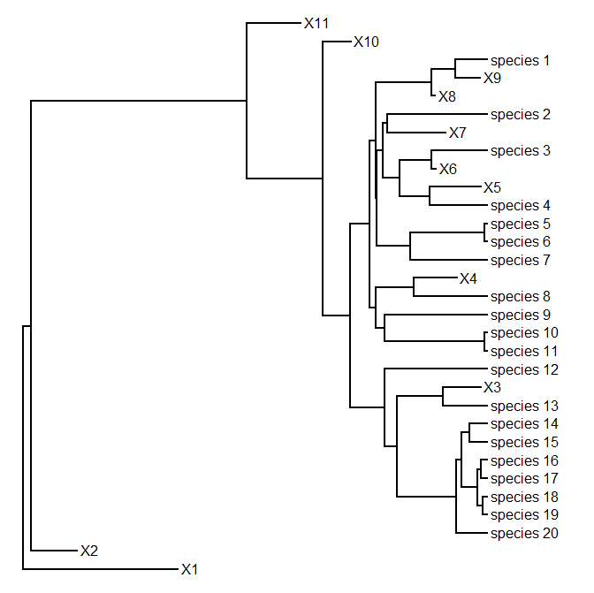
> plotTree(tree)
> tree<-pbtree(b=1,d=0.3,n=20,tip.label=paste("species_", 20:1,sep=""))
Warning: only using labels in tip.label for extant tips.
extinct tips will be labeled X1, X2, etc.
> plotTree(tree)
> ## this will probably go completely extinct
> tree<-pbtree(b=1,d=0.9,n=10,tip.label=letters[1:10])
Warning: only using labels in tip.label for extant tips.
extinct tips will be labeled X1, X2, etc.
> plotTree(tree)
> ## n & t
> n<-26
> b<-1
> d<-0.4
> t<-log(26/2)/(b-d)
> tree<-pbtree(n=n,t=t,b=b,d=d,tip.label=LETTERS[26:1], method="direct")
Warning: only using labels in tip.label for extant tips.
extinct tips will be labeled X1, X2, etc.
simulating with both taxa-stop (n) & time-stop (t) using
'direct' sampling. this is experimental
> plotTree(tree)

Simulating DNA sequences with Γ rate heterogeneity among sites

$
0
0

I just added this to the (fairly maligned) function genSeq, for simulating DNA sequences by (inefficiently) wrapping the phytools function sim.history. Here's what the function looks like now:

genSeq<-function(tree,l=1000,Q=NULL,rate=1, format="DNAbin",...){
 if(is.null(Q)){
  Q<-matrix(1,4,4)
  rownames(Q)<-colnames(Q)<-c("a","c","g","t")
  diag(Q)<-0
  diag(Q)<--colSums(Q)
 }
 if(length(rate)!=l){
  if(length(rate)==1) rate<-rep(rate,l)
  else {
   cat("warning: length(rate) & l should match for      length(rate)>1\n")
   cat(" rate will be recycled.\n")
   rate<-rep(rate,ceiling(l/length(rate)))[1:l]
  }
 }
 cat("simulating sequences....\n")
 X<-sapply(rate,function(a,b,c)   sim.history(b,a*c)$states,b=tree,c=Q)
 if(format=="DNAbin") return(as.DNAbin(X))
 else if(format=="phyDat") return(as.phyDat(X))
 else if(format=="matrix") return(X)
}

One can easily see that the way rate heterogeneity is handled is by allowing the user to supply a site-specific vector of rates. Here's what this would look like if we wanted to simulate sequences under a continuous Γ rate heterogeneity model with a shape parameter, α = 0.25 and a mean rate of 1.0 substitution per site per unit of branch length:

> library(phytools)
> tree<-pbtree(n=26,tip.label=LETTERS,scale=0.1)
> gg<-rgamma(n=1000,shape=0.25,rate=0.25)
> X<-genSeq(tree,rate=gg)
simulating sequences....
> X
26 DNA sequences in binary format stored in a matrix.

All sequences of same length: 1000

Labels: A B C D E F ...

Base composition:
    a    c    g    t
0.264 0.245 0.242 0.249

We can do invariant sites the same way - although in this case it will break the function if we set any of the rates to zero, so we need to set them very slightly > 0:

> ii<-rep(1,1000)
> tol<-1e-12
> ii[sample(1:1000,100)]<-tol
> X<-genSeq(tree,rate=ii)
simulating sequences....
> X
26 DNA sequences in binary format stored in a matrix.

All sequences of same length: 1000

Labels: A B C D E F ...

Base composition:
    a    c    g    t
0.244 0.261 0.238 0.257

As Klaus pointed out, this method is very slow - so you probably have better options. But it's still a fun exercise to see how it works - and offers the interesting possibility that we could store and return all character histories along with the states for tips.

Coloring tip labels by character state

$
0
0

Yesterday I received the query:

"I want to color my tree tip labels according to a particular character and provide a legend for the same."

Here's a demo of one way to do this, using the phytools data object anoletree:

require(phytools)
data(anoletree)
tree<-anoletree
x<-getStates(tree,"tips")
par(fg="transparent")
plotTree(tree,fsize=0.6,ylim=c(-1,length(tree$tip.label)))
lastPP<-get("last_plot.phylo",env=.PlotPhyloEnv)
ss<-sort(unique(x))
colors<-setNames(palette()[1:length(ss)],ss)
par(fg="black")
add.simmap.legend(colors=colors,vertical=FALSE,x=0.25,
  y=-1,prompt=FALSE)
colors<-sapply(x,function(x,y) y[which(names(y)==x)],
  y=colors)
tt<-gsub("_","",tree$tip.label)
text(lastPP$xx[1:length(tt)],lastPP$yy[1:length(tt)],
  tt,cex=0.6,col=colors,pos=4,offset=0.1,font=3)

Here's the result:

Obviously, some of this is idiosyncratic to this specific dataset. Hopefully, users can figure out how to modify this to their own data and problem.

Plotting phylogenies with triangles for subtrees

$
0
0

Here's something new. Luke Mahler asked me if I could create a plotting method that could take a backbone phylogeny and plot subtrees using triangles that are scaled proportionally to the number of species in the subtree. I'm still working on this, but I posted some preliminary code here.

The function takes a modified tree as an object of class "backbonePhylo". I'm going to make some functions to convert from "phylo" objects, but for now this has to be built manually. The "backbonePhylo" object is like a "phylo" object, but with tip.clade substituted for tip.label. tip.clade is a list in which each subtree is represented by a label, a number of descendant taxa, and crown group depth.

Here's a quick demo of what can be done so far:

> library(phytools)
> library(geiger) # to help us build our tree
> source("backbonePhylo.R")
> ## now let's create our backbone tree with
> ## random subtree diversities
> tree<-transform(pbtree(n=10),model="lambda",lambda=0.5)
> tree$tip.clade<-list()
> for(i in 1:10){
  tree$tip.clade[[i]]<-
    list(label=paste("Group",i),
    N=ceiling(runif(n=1,min=0,max=20)),
    depth=tree$edge.length[which(tree$edge[,2]==i)])
  }
> class(tree)<-"backbonePhylo"
> tree

Backbone phylogenetic tree with 10 subtrees and 9 resolved internal nodes.

Labels: Group 1, Group 2, Group 3, Group 4, Group 5, ...
Diversities: 2, 18, 13, 7, 9, ...

> ## ok, let's plot it
> plot(tree)

Cool. That's more or less what we were going for.

More on plotting backbone trees with triangles as subtrees

$
0
0

Yesterday (more accurately, early this morning), I posted about a new plotting method for plotting a backbone phylogeny with diversities for each subtree represented as a triangle. This type of visualization is quite common in the literature; however, I'm told (by Luke Mahler, so blame him if this is incorrect) that there is no such plotting method so far in R.

The way I did this was by first creating a new type of phylogeny object, of class "backbonePhylo". This object is stored in a very similar way to the typical phylogeny object in R (class "phylo"), which the exception that we have replaced the vector tip.label with the list tip.clade. tip.clade is a list in which each element contains a label, a diversity (i.e., the number of tips hidden in the subtree), and a crown depth.

I have written some of the methods around this object as S3 methods, which means they can be dispatched using (for instance) calls to the generic plot, reorder, print, etc.

This morning, I did a little more work on this suite of functions. Most importantly, I created a new function (phylo.toBackbone) that converts an object of class "phylo" to an object of class "backbonePhylo" with the help of a translation table. The translation table is a data frame with four variables: tip.label (containing the names of the tips in the input tree - these might be exemplar taxa); label (containing the names of the subtrees - these might be the names of higher taxa); N (obviously, the diversities of each subtree); and depth (the age of each crown group, in terms of the branch lengths of the input tree - note that this cannot be longer then the corresponding tip edge). Note that not all tips in the original tree need to be in the translation table. Those that are not will be treated as clades containing one taxon in the backbone tree.

Here's a demo using random subtree sizes on a stochastic backbone tree. New code for this is here.

> library(phytools)
> library(geiger) # to help us build our tree
> source("backbonePhylo.R")
> ## now let's create our backbone tree
> tree<-transform(pbtree(n=10),model="lambda",lambda=0.5)
> ## for old versions of geiger, use lambdaTree
>
> ## create a translation table
> ## leaving a couple of single-taxon clades for fun
> tip.label<-sample(tree$tip.label,8)
> clade.label<-LETTERS[1:8]
> N<-ceiling(runif(n=8,min=1,max=20))
> ## set crown node depth to 1/2 the maximum depth
> depth<-sapply(tip.label,function(x,y) 0.5*y$edge.length[which(tree$edge[,2]==which(y$tip.label== x))],y=tree)
> trans<-data.frame(tip.label,clade.label,N,depth)
> rownames(trans)<-NULL
> rm(tip.label,clade.label,N,depth)
>
> ## here's what trans looks like
> trans
  tip.label clade.label  N    depth
1        t2           A  6 0.8992932
2        t4           B  5 0.7617329
3        t3           C 16 0.8674696
4        t5           D  9 0.5984337
5        t1           E  5 0.8992932
6       t10           F  7 0.5554955
7        t7           G  8 0.5664347
8        t9           H  7 0.5554955
>
> ## convert
> tt<-phylo.toBackbone(tree,trans)
>
> ## plot
> plot(tt)

That's pretty good.

Even more on plotting subtrees as triangles on a phylogenetic backbone tree

$
0
0

This is pretty much guaranteed to be the last post on this topic today, but I made some additional refinements of plot.backbonePhylo, my new plotting method to show subtrees as triangles.

The three main changes are as follows: (1) following Luke's suggestion, subtrees containing only 1 taxon are now plotted as a line (actually - a triangle with zero width, but I guarantee you won't be able to tell the difference), instead of as a triangle with unit width; (2) following Graham Slater's suggestion, I made a small change so that there is a space between adjacent triangles - the consequence is that clades with 2 taxa are of unit length, clades with 10 taxa are 9 units in width, etc., which actually lines up with tips containing 1 taxon, which now have unit width; and (3) I added the optional scaling factor vscale, which scales the vertical dimension so that large subtrees can be portrayed while still allowing singletons and spacing between triangles.

All of these updates are available here, but are also part of a new phytools build (phytools 0.3-51).

Here's a demo:

> library(phytools)
> packageVersion("phytools")
[1] ‘0.3.51’
> library(geiger) # to help us build our tree
> ## now let's create our backbone tree with
> ## random subtree diversities
> tree<-transform(pbtree(n=10),model="lambda",lambda=0.5)
> ## for old versions of geiger, use lambdaTree
>
> ## create a translation table
> ## leaving a couple of single-taxon clades for fun
> tip.label<-sample(tree$tip.label,8)
> clade.label<-LETTERS[1:8]
> N<-ceiling(runif(n=8,min=1,max=20))
> ## set crown node depth to 1/2 the maximum depth
> depth<-sapply(tip.label,function(x,y) 0.5*y$edge.length[which(tree$edge[,2]==which(y$tip.label== x))],y=tree)
> trans<-data.frame(tip.label,clade.label,N,depth)
> rownames(trans)<-NULL
> rm(tip.label,clade.label,N,depth)
>
> ## here's what trans looks like
> trans
  tip.label clade.label  N     depth
1        t4           A  3 1.0079214
2        t8           B 13 0.8367549
3        t1           C 15 1.1433276
4        t3           D  8 1.0129504
5        t6           E 12 0.9687320
6        t5           F  2 0.9687320
7        t9           G 14 0.7253729
8       t10           H 17 0.7253729

> ## convert
> tt<-phylo.toBackbone(tree,trans)
>
> ## plot
> plot(tt)
> ## now let's make our clades much bigger
> trans$N<-trans$N*10
> trans
  tip.label clade.label   N     depth
1        t4           A  30 1.0079214
2        t8           B 130 0.8367549
3        t1           C 150 1.1433276
4        t3           D  80 1.0129504
5        t6           E 120 0.9687320
6        t5           F  20 0.9687320
7        t9           G 140 0.7253729
8       t10           H 170 0.7253729
> tt<-phylo.toBackbone(tree,trans)
> plot(tt)
> ## now let's use the new parameter vscale
> plot(tt,vscale=0.1)

Pretty cool.

We have to be careful with this, though, because if we adjust our clade widths such that any are less than 1 unit then we are going to get some really weird plots.

Getting Robinson-Foulds distances for a set of trees

$
0
0

The phangorn function RF.dist - for computing the Robinson-Foulds distance between two trees - is very fast. However if we want to compare a set of trees stored in an object of class "multiPhylo" there is some opportunity to recycle internal calculations & thus improve on just calling RF.distn× (n - 1) / 2 times for n trees. Specifically, here is some code that scales to multiple trees a little bit better than n× (n - 1) / 2 RF.dist by calling the ape function prop.part (which finds all bipartitions in the tree) only once for each tree:

multiRF<-function(trees){
 if(class(trees)!="multiPhylo")
  stop("trees should be an object of class \"multiPhylo\"")
 N<-length(trees)
 RF<-matrix(0,N,N)
 if(any(sapply(unclass(trees),is.rooted))){
  cat("Some trees are rooted. Unrooting all trees.\n")
  trees<-lapply(unclass(trees),unroot)
 }
 foo<-function(pp) lapply(pp,function(x,pp)
  sort(attr(pp,"labels")[x]),pp=pp)
 xx<-lapply(unclass(trees),function(x) foo(prop.part(x)))
 for(i in 1:(N-1)) for(j in (i+1):N)
  RF[i,j]<-RF[j,i]<-2*sum(!xx[[i]]%in%xx[[j]])
 RF
}

It works OK compared to calling RF.dist a whole bunch of times independently. First, here is an alternate version of the function which uses RF.dist:

multiRF2<-function(trees){
 N<-length(trees)
 RF<-matrix(0,N,N)
 for(i in 1:(N-1)) for(j in (i+1):N)
  RF[i,j]<-RF[j,i]<-RF.dist(trees[[i]],trees[[j]])
 RF
}

Now, a very simple comparison with random trees:

> N<-100
> n<-100
> trees<-rmtree(N,n,rooted=FALSE)
> system.time(X1<-multiRF(trees))
   user  system elapsed
   9.16    0.03    9.19
> system.time(X2<-multiRF2(trees))
   user  system elapsed
  19.98    0.00   19.99
> all(X1==X2)
[1] TRUE

Slightly faster multiple pairwise RF distance

$
0
0

I just posted a slightly faster version of multiRF that takes advantage of the fact that the first element in the list of tree bipartitions from prop.part of the ape package is the "partition" with all the taxa in the tree - which can be ignored if our two input trees have the same taxa (they should). The result is about a 20% speed-up in the 100 × 99 ÷ 2 comparisons for 100, 100-taxon trees.

Here's a demo using my i3 Asus Vivobook (obviously - it would be much faster on a speedy desktop):

> library(phytools)
> library(phangorn)
> packageVersion("phytools")
[1] ‘0.3.53’
> ## circumvents rNNI from phangorn which is buggy
> ## in the current version
> randomNNI<-function(tree,moves=1){
  for(i in 1:moves) tree<-sample(nni(tree),1)[[1]]
  tree
 }
> ## random tree
> tree<-rtree(n=100,rooted=FALSE,br=NULL)
> ## 100 trees random NNIs
> trees<-lapply(round(runif(n=100,min=1,max=100)), function(x,y) randomNNI(y,x),y=tree)
> class(trees)<-"multiPhylo"
> ## this is a hack
> trees<-read.tree(text=write.tree(trees))
> ## compute all pairwise RF
> system.time(D1<-multiRF(trees))
   user  system elapsed
  16.41    0.02   16.58
> ## now compare to new version
> detach("package:phytools",unload=TRUE)
> install.packages("phytools_0.3-60.zip",repos=NULL)
package ‘phytools’ successfully unpacked and MD5 sums checked
> library(phytools)
> packageVersion("phytools")
[1] ‘0.3.60’
> system.time(D2<-multiRF(trees))
   user  system elapsed
  13.28    0.01   13.29
> plot(D1,D2)
(Just to verify that it still works!)

BTW, I just submitted phytools 0.3-60 to CRAN - so hopeful it is accepted & percolates through the mirror repositories this week.


Computing the residuals for individuals from phylogenetic regression

$
0
0

A little while ago I received the following query:

"To account for body size I used the phylogenetic regression of your phyl.resid function. I used the mean value of each trait per species. However, now I would like to plot the residuals against the ecological variables to show how they relate, including standard deviations for trait means. Is there a way to calculate phylogenetically corrected residuals with standard deviations? Or simply calculate residuals for more than one individual per species?"

Well, there are multiple ways we could go about doing this - with multiple possible solutions. The simplest thing, and the one I'd probably recommend for starters, is to fit the phylogenetic regression to and , the species means vectors; but then compute = [1 x]β and e = y - from the original data vectors, x&y.

Here's how that would look if we had input data vectors xi and yi, both with the same order but in which names(xi) and names(yi) contain only species names (& thus no unique identifiers):

## first aggregate xi & yi to compute species means
xbar<-aggregate(xi,by=list(names(xi)),FUN=mean)
xbar<-setNames(xbar[,2],xbar[,1])
ybar<-aggregate(yi,by=list(names(yi)),FUN=mean)
ybar<-setNames(ybar[,2],ybar[,1])
## now fit PGLS model
fit<-gls(ybar~xbar,data.frame(xbar,ybar),correlation=
  corBrownian(1,tree))
## compute yhat based on individual data in xi
yhat<-(cbind(1,xi)%*%fit$coef)[,1]
## compute individualized residuals
ei<-yi-yhat

Note that the species-wise mean of ei will be exactly equal to our residuals from the fitted model using species means. E.g., compare:

ebar<-aggregate(ei,by=list(names(ei)),FUN=mean)
ebar<-setNames(ebar[,2],ebar[,1])
## with
residuals(fit)
They should be the same.

That's it!

Finding the edge lengths of all the terminal branches in the tree

$
0
0

A phytools user asks:

"I have a list of names that correspond exactly to the tips of a phylogenetic tree. What i'd like to do is obtain the branch lengths that correspond to these tip edges."

This can be done with one line:

n<-length(tree$tip.label)
ee<-setNames(tree$edge.length[sapply(1:n,function(x,y)   which(y==x),y=tree$edge[,2])],tree$tip.label)
(Or at least this would be one line if the width of this entry window permitted me to put length(tree$tip.label) into my sapply block instead of first calculating n.)

We get a vector with all the terminal edge lengths with names set to all the tip names in the tree, so we can rearrange or select a subset of these tip lengths on that basis.

Let's check it:

> tree<-pbtree(n=10)
> tree$edge.length<-round(tree$edge.length,3)
> n<-length(tree$tip.label)
> ee<-setNames(tree$edge.length[sapply(1:n,function(x,y) which(y==x),y=tree$edge[,2])],tree$tip.label)
> ee
   t9   t10    t3    t4    t7    t8    t2    t1    t5    t6
0.262 0.262 0.587 0.587 0.385 0.385 0.641 0.727 0.432 0.432
> plotTree(tree)
> edgelabels(tree$edge.length)

Optimizing pgls.Ives with Pagel's λ

$
0
0

Today I got the following interesting user request:

"I have been playing around with the function pgls.Ives. Is there anyway to accomodate the corPagel correlation structures into this?"

This is not possible, actually. corStruct objects (such as an object of class "corPagel") do not permit (so far as I know) error in both x & y which is a component of the pgls.Ives model. However we can, with a little pain, optimize Pagel's λ model using pgls.Ives - just in a slightly roundabout way. We do this by building a simple wrapper around pgls.Ives that spits out the log-likelihood conditioned on a specific input λ, then we optimize for λ. Here's a demo:

## load packages & simulate data
require(phytools)
require(geiger)

# simulate tree & data under the regression model
tree<-pbtree(n=50)
xhat<-fastBM(tree)
yhat<-0.75*xhat+0.2*fastBM(transform(tree,lambda=0.5))

# simulate individual data for x & y
x<-sampleFrom(xhat,randn=c(1,10))
n<-summary(as.factor(names(x)))
y<-sampleFrom(yhat,n=n[names(yhat)])
Now let's fit the model using λ:
## brute force grid search optimization
lambda<-seq(0.05,1,0.05)
logL<-sapply(lambda,function(l,tree,x,y)
  pgls.Ives(transform(tree,lambda=l),x,y)$logL,tree=tree,
  x=x,y=y)
ii<-which(logL==max(logL))
plot(lambda,logL,type="b")
lines(c(lambda[ii],lambda[ii]),c(min(logL),max(logL)),
  lty="dashed")
ml.lambda<-lambda[ii]
ml.lambda

## optimize using base function optimize
foo<-function(l,tree,x,y)
  pgls.Ives(transform(tree,lambda=l),x,y)$logL
optimize(foo,c(0,1),tree=tree,x=x,y=y,maximum=TRUE)

Let's try it:

> # simulate tree & data under the regression model
> tree<-pbtree(n=50)
> xhat<-fastBM(tree)
> yhat<-0.75*xhat+0.2*fastBM(transform(tree,lambda=0.5))
>
> # simulate individual data for x & y
> x<-sampleFrom(xhat,randn=c(1,10))
> n<-summary(as.factor(names(x)))
> y<-sampleFrom(yhat,n=n[names(yhat)])
>
> ## brute force grid search optimization
> lambda<-seq(0.05,1,0.05)
> logL<-sapply(lambda,function(l,tree,x,y)
pgls.Ives(transform(tree,lambda=l),x,y)$logL,tree=tree,
x=x,y=y)
There were 50 or more warnings (use warnings() to see the first 50)
> ii<-which(logL==max(logL))
> ml.lambda<-lambda[ii]
> ml.lambda
[1] 0.7
> plot(lambda,logL,type="b")
> lines(c(lambda[ii],lambda[ii]),c(min(logL),max(logL)),
lty="dashed")
> ## optimize using base function optimize
> foo<-function(l,tree,x,y) pgls.Ives(transform(tree,lambda=l),x,y)$logL
> optimize(foo,c(0,1),tree=tree,x=x,y=y,maximum=TRUE)
$maximum
[1] 0.6893112

$objective
[1] -134.8

There were 42 warnings (use warnings() to see them)
The warnings, in this case, are just that the sample sizes for some species are one - so the function assumes that that species has a within species variance equal to the mean variance across all species.

Note that although this works fine in principle, I have received some reports of the basic function failing to optimize for larger trees - and I believe these reports, so please use pgls.Ives with considerable caution until I work out these issues!
Simplified lambdaTree

$
0
0

I'm running some tests on phytools right now to try and put a new version on CRAN, but one of them required I use the function lambdaTree in the geiger package. geiger is not a dependency of phytools, so I wanted to be able to do this (ideally) without loading geiger. Here is a simplified lambdaTree (now deprecated into transform.phylo):

lambdaTree<-function(tree,lambda){
  ii<-which(tree$edge[,2]>length(tree$tip.label))
  H1<-nodeHeights(tree)
  tree$edge.length[ii]<-lambda*tree$edge.length[ii]
  H2<-nodeHeights(tree)
  tree$edge.length[-ii]<-tree$edge.length[-ii]+     H1[-ii,2]-H2[-ii,2]
  tree
}

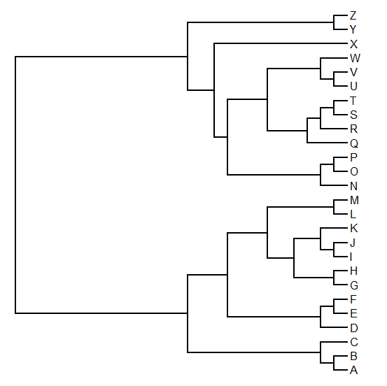
Here's a quick check:

> library(geiger)
> library(phytools)
> tree<-pbtree(n=26,tip.label=LETTERS[26:1])
> plotTree(transform(tree,model="lambda",lambda=0.5), mar=c(0,1,4,1))
> title(main="a) transform.phylo",adj=0)
> plotTree(lambdaTree(tree,0.5),mar=c(0,1,4,1))
> title(main="b) simple lambdaTree",adj=0)

New version of phytools on CRAN

$
0
0

A new version of phytools (phytools 0.3-72) is now on CRAN. It's been a few months since the previous CRAN version. This is partly because I had to do some work on the minor phytools versions that I've been posting to bring them into compliance with changing CRAN standards. For instance, CRAN now encourages functions that are used in package dependencies to also be imported using importFrom in the NAMESPACE file, and foreign function calls to compiled C code in other packages are no longer generally permitted (or, at least, they are actively discouraged).

Here's a (possibly non-comprehensive) list of updates/new functions/etc. in the current CRAN version of phytools relative to the last CRAN release (phytools 0.3-10):

1. An update to phyl.cca that results when spectral decomposition produces slightly negative eigenvalues (due to limitations on numerical precision) for a positive semi-definite covariance matrix.

2. An update to densityMap to allow users to plot the variation among stochastic maps.

3. A new function (phylo.to.map, and S3 plotting method) to visual a phylogeny connected to or projected onto a geographic map (1, 2, 3).

4. A new version of mergeMappedStates to merge two or more mapped states on a stochastic map tree.

5. A new function (drop.leaves) to strip all the leaves off of a phylogenetic tree.

6. A new version of ancThresh (for ancestral character estimation under the threshold model) which also permits us to fit an OU model for the evolution of liability on the tree.

7. Major updates to the innards of the important phytools plotting function plotSimmap.

8. An update to plotSimmap(...,type="fan") to permit node labels.

9. A new 'static' plotting method for phylomorphospace3d.

10. A new version of plotTree that will supply branch lengths using compute.brlen in 'ape' if none are provided.

11. An update to bmPlot(...,type="threshold") which also maps the (discrete generation) history of a threshold character on the branches of a phylogeny & returns this tree to the user.

12. A new function (map.to.singleton) that converts a tree with a mapped character to a tree with singleton nodes; and a new plotting method (plotTree.singletons) for plotting these trees.

13. A new version of contMap (and, in fact, densityMap) to allow users to plot left-facing trees.

14. A simple DNA evolution simulator (genSeq) that wraps around sim.history (1, 2).

15. A new version of pbtree that allows user-defined tip labels.

16. A new set of methods to plot a backbone phylogeny with triangles as subtrees (1, 2, 3).

17. A new function (multiRF) for computing all pairwise Robinson-Foulds distances for a set of trees that recycles internals to be slightly speedier (1, 2).

18. Additional minor updates to branching.diffusion, xkcdTree, anc.trend, phylomorphospace3d, strahlerNumber, and map.to.singleton.

19. Minor updates to the documentation of various functions.

In addition to these changes, and as I alluded above, I made a bunch of additional updates (that will generally be hidden to the user) to the way phytools depends on other packages. I did this primarily to bring phytools into compliance with evolving CRAN standards. Hopefully none of these changes affect phytools users adversely.

Obviously, keep in mind that it may take a few days for Mac & Windows phytools binaries to be build & for the updated version of phytools to percolate through all the CRAN mirrors.

Thanks for using phytools!

Viewing all 802 articles
Browse latest View live