Since our second Latin American Macroevolution workshop - this year held in Ilhabela, Brazil - is now done, I thought I'd post a quick update on our final t-shirt design. I posted a prototypical version earlier on this blog; however subsequent to making that design we decided to switch from a continuous character map, so a stochastically mapped discrete character using a Brazilian flag color palette. Here is the result:

library(phytools)
## read in tree
tree<-read.tree(text="(((t2:0.41,((t15:0.116,(t68:0.03,t69:0.03):0.086):0.18,(((t43:0.058,((t97:0.001,t98:0.001):0.03,t67:0.032):0.027):0.072,((t95:0.002,t96:0.002):0.028,t70:0.03):0.1):0.072,t5:0.202):0.094):0.114):0.004,((((((t76:0.022,t77:0.022):0.05,(t61:0.034,t62:0.034):0.038):0.03,((t91:0.005,t92:0.005):0.021,t75:0.026):0.076):0.083,t9:0.185):0.2,(((t10:0.16,((t30:0.078,(t80:0.014,t81:0.014):0.064):0.005,((((t99:0,t100:0):0.03,(t73:0.027,t74:0.027):0.004):0.004,t60:0.034):0.011,t51:0.045):0.038):0.077):0.054,(t7:0.188,(((t54:0.039,(t84:0.01,t85:0.01):0.028):0.09,t14:0.129):0.027,(t31:0.076,(t57:0.034,t58:0.034):0.042):0.08):0.032):0.026):0.083,(((t93:0.004,t94:0.004):0.002,t90:0.006):0.204,((t71:0.029,t72:0.029):0.101,t13:0.13):0.08):0.086):0.088):0.024,((t3:0.26,(t4:0.207,((t32:0.074,(t49:0.049,t50:0.049):0.026):0.099,(((((t78:0.018,t79:0.018):0.025,t52:0.042):0.054,t21:0.096):0.034,t12:0.13):0.01,(t33:0.074,((t65:0.032,t66:0.032):0.009,t53:0.041):0.032):0.067):0.032):0.034):0.053):0.016,(t11:0.154,(t26:0.086,((t55:0.036,t56:0.036):0.018,t46:0.054):0.032):0.068):0.122):0.132):0.004):0.086,((((t8:0.186,((t16:0.114,(t24:0.088,t25:0.088):0.027):0.008,(t40:0.068,t41:0.068):0.054):0.063):0.08,(((((t47:0.051,t48:0.051):0.044,t22:0.095):0.009,t18:0.104):0.053,((t19:0.102,((t83:0.012,(t86:0.01,t87:0.01):0.002):0.054,t42:0.068):0.034):0.018,((t23:0.09,(t28:0.085,t29:0.085):0.005):0.011,(t38:0.068,t39:0.068):0.034):0.018):0.038):0.03,((t44:0.057,t45:0.057):0.048,t17:0.104):0.082):0.08):0.082,(((t59:0.034,(t82:0.014,(t88:0.009,t89:0.009):0.004):0.021):0.13,(((t34:0.073,t35:0.073):0.013,t27:0.086):0.015,(t63:0.033,t64:0.033):0.068):0.064):0.059,(t6:0.19,((t36:0.072,t37:0.072):0.028,t20:0.1):0.09):0.033):0.125):0.098,t1:0.446):0.054);")
## create transition matrix
Q<-matrix(c(-3,1,1,1,
    1,-3,1,1,
    1,1,-3,1,
    1,1,1,-3),4,4)
rownames(Q)<-colnames(Q)<-letters[1:4]
## simulate stochastic character history
tree<-sim.history(tree,Q)

## Done simulation(s).

cols<-setNames(c("#309030","#182B78","#F0F0F0","#F0C000","#134913"),
    letters[1:4])

Now we're ready to make our plot:

layout(mat=matrix(c(1,2),2,1),heights=c(0.8,0.2))
par(bg="black")
par(fg="white")
plotSimmap(paintSubTree(tree,Ntip(tree)+1,"1"),type="fan",
    ftype="off",colors=setNames("white","1"),lwd=6,part=0.5)

## setEnv=TRUE for this type is experimental. please be patient with bugs

plotSimmap(tree,colors=cols,type="fan",ftype="off",lwd=4,
    add=TRUE,part=0.5)

## setEnv=TRUE for this type is experimental. please be patient with bugs

plot.new()
text(0.5,0.5,"Latin American Macroevolution Workshop\nIlhabela Brazil 2015",
    col="white",cex=2.1,font=2)

Once again, if we want to produce a high quality version without the aliasing that we see in the plot above, we can do that easily by exporting as a pdf:

pdf(file="brazil-colors.pdf",width=8,height=4.75)
layout(mat=matrix(c(1,2),2,1),heights=c(0.8,0.2))
par(bg="black")
par(fg="white")
plotSimmap(paintSubTree(tree,Ntip(tree)+1,"1"),type="fan",
    ftype="off",colors=setNames("white","1"),lwd=6,part=0.5)

## setEnv=TRUE for this type is experimental. please be patient with bugs

plotSimmap(tree,colors=cols,type="fan",ftype="off",lwd=4,
    add=TRUE,part=0.5)

## setEnv=TRUE for this type is experimental. please be patient with bugs

plot.new()
text(0.5,0.5,"Latin American Macroevolution Workshop\nIlhabela Brazil 2015",
    col="white",cex=2.1,font=2)
dev.off()

## png 
##   2

This PDF can be found here.

Note that since the plot above used a stochastic simulation, the realized t-shirt design was actually slightly different (see below).

Finally, the course was a huge success (in my opinion). Certainly, the students we had this year (like last year) were fantastic, and they even seemed to like the t-shirts:

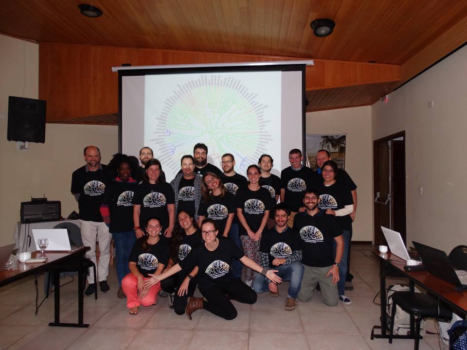
(Click for a larger version.)

Thanks to the TAs, my co-instructors Luke Harmon & Mike Alfaro, and, of course, the excellent students. We're already looking forward to next year!

I just added a function to plot co-phylogenetic trees (that is, trees which have been plotted to maximize the vertical alignment of tips). This is not meant to displace or replace the function cophyloplotfrom the ape package, just as an alternative. It also does not (yet) contain the full range of plotting options that can be accesses using (for example) plot.phylo or plotSimmap (neither of which are used internally by this function. Consequently, though the function produces a nice visualization (in my opinion) - it is not particularly flexible.

It works in the following way. First, the function cophylotakes two trees and an “association” table to (by default) try to rotate all the nodes of the tree so that the match the specified association as closely as possible. It returns an object of class "cophylo"which is then plotted using an S3 plotting method that I have written for that object class.

Here is a demo using a simulated tree & association matrix:

library(phytools)
source("http://www.phytools.org/cophylo/v0.1/cophylo.R")
N<-20
tips.tr1<-replicate(N,paste(sample(LETTERS,1),"._",
    paste(sample(letters,round(runif(n=1,min=4,max=8))),
    collapse=""),sep=""))
tips.tr2<-replicate(N,paste(sample(LETTERS,1),"._",
    paste(sample(letters,round(runif(n=1,min=4,max=8))),
    collapse=""),sep=""))
tr1<-pbtree(n=N,tip.label=tips.tr1)
tr2<-pbtree(n=N,tip.label=sample(tips.tr2))
assoc<-cbind(tips.tr1,tips.tr2)
## here is our association matrix
assoc

##       tips.tr1      tips.tr2     
##  [1,] "W._dlwm"     "A._fzgam"   
##  [2,] "X._escrndyh" "W._szwf"    
##  [3,] "E._bqnfgamo" "S._yxau"    
##  [4,] "U._flhus"    "X._awegv"   
##  [5,] "A._wtidb"    "P._xeiuglq" 
##  [6,] "E._fgcjur"   "P._fpoqim"  
##  [7,] "D._dvsnroq"  "C._otvsn"   
##  [8,] "B._ampg"     "P._mxbra"   
##  [9,] "S._jtugw"    "Y._nqum"    
## [10,] "F._lkein"    "K._qvrml"   
## [11,] "D._wsahm"    "J._ecslngd" 
## [12,] "K._tjwybe"   "R._vxedtwu" 
## [13,] "W._kesxcfy"  "J._vycwi"   
## [14,] "J._dluaog"   "S._pebgjt"  
## [15,] "O._widztm"   "N._gjeklr"  
## [16,] "R._iabcfg"   "O._yhmpdwle"
## [17,] "U._vykna"    "V._evuls"   
## [18,] "L._krumtvwa" "J._tzocbar" 
## [19,] "R._gitlsuy"  "B._imgyxv"  
## [20,] "K._yajemc"   "X._vctdwuf"

Now let's run our functions. First without rotation, then with rotation (the default):

## no rotation
obj<-cophylo(tr1,tr2,rotate=FALSE,assoc=assoc)
obj

## Object of class "cophylo" containing:
## 
## (1) 2 (possibly rotated) phylogenetic trees in an object of class "multiPhylo".
## 
## (2) A table of associations between the tips of both trees.

plot(obj)

## with rotation
obj<-cophylo(tr1,tr2,assoc=assoc)
obj

## Object of class "cophylo" containing:
## 
## (1) 2 (possibly rotated) phylogenetic trees in an object of class "multiPhylo".
## 
## (2) A table of associations between the tips of both trees.

plot(obj)

If we don't specify an association matrix, then the function assumes that the tip labels are meant to match exactly. We also do not need to use trees that are ultrametric. Here is an example that demonstrates both points:

tr1<-rtree(n=30)
tr2<-rtree(n=30)
obj<-cophylo(tr1,tr2)
plot(obj)

That's it!

Today I have continued to play around with the method I posted yesterdayto create a kind of “co-phylogenetic plot” - that is, a plot of left & right facing phylograms with the tips lined up, & connected, so as to show an association between species.

The major improvements that I made are the following:

(1) I improved the tip rotation optimization method, and now allow the user to specify a function for the optimization (such as function(x) x2, which tells cophylo to minimize the sum of squares deviations between the plots; or function(x) abs(x), which tells it to minimize the summed absolute values.

(2) I now permit the trees to have different numbers of tips and thus incomplete matching (some taxa in one or the other trees that have no match in the second).

(3) When no assoc matrix is supplied, cophylonow checks for any taxa with matching labels between the two trees, not just to see if all tip labels match.

(4) Now, one tip in one tree can match to multiple tips in a second (and/or vice versa).

Finally, (5) if no associations are provided (& none can be found), the function simply returns two facing trees to be plotted by plot.cophylo.

In the previous version of this function I was using a slightly modified version of the phytools function minRotateto perform the node rotation optimization. I have replaced this with a custom internal function which is much more flexible and better suited to this particular task.

Here's a demo of some of this functionality:

library(phytools)
source("http://www.phytools.org/cophylo/v0.2/cophylo.R")

First, the basic usage, but specifying different functions to optimize node rotation. The default is x2.

tr1<-pbtree(n=26,tip.label=LETTERS)
tr2<-pbtree(n=26,tip.label=sample(LETTERS))
obj<-cophylo(tr1,tr2,rotate=FALSE)
plot(obj)

obj<-cophylo(tr1,tr2)

## Rotating nodes to optimize matching...
## Done.

plot(obj)

obj<-cophylo(tr1,tr2,fn=function(x) abs(x))

## Rotating nodes to optimize matching...
## Done.

plot(obj)

Now, multiple one tip in tr1 match to multiple tips in tr2 and vice versa:

assoc<-cbind(c("A","A","A","X","Y","Z"),
    c("A","B","C","Z","Z","Z"))
assoc

##      [,1] [,2]
## [1,] "A"  "A" 
## [2,] "A"  "B" 
## [3,] "A"  "C" 
## [4,] "X"  "Z" 
## [5,] "Y"  "Z" 
## [6,] "Z"  "Z"

obj<-cophylo(tr1,tr2,assoc,rotate=FALSE)
plot(obj)

obj<-cophylo(tr1,tr2,assoc)

## Rotating nodes to optimize matching...
## Done.

plot(obj)

Now, a partial matching of tip labels between trees:

tr1<-pbtree(n=12,tip.label=sample(LETTERS[1:12]))
tr2<-pbtree(n=12,tip.label=sample(LETTERS[7:18]))
obj<-cophylo(tr1,tr2)

## Rotating nodes to optimize matching...
## Done.

plot(obj)

Trees with different numbers of tips and partial matching:

tr1<-rtree(n=40)
tr2<-rtree(n=26,tip.label=LETTERS)
assoc<-cbind(sample(tr1$tip.label,20),sample(LETTERS,20))
assoc

##       [,1]  [,2]
##  [1,] "t25" "U" 
##  [2,] "t12" "Z" 
##  [3,] "t37" "A" 
##  [4,] "t22" "N" 
##  [5,] "t39" "H" 
##  [6,] "t9"  "L" 
##  [7,] "t8"  "K" 
##  [8,] "t23" "D" 
##  [9,] "t33" "W" 
## [10,] "t18" "X" 
## [11,] "t1"  "P" 
## [12,] "t4"  "G" 
## [13,] "t5"  "V" 
## [14,] "t19" "T" 
## [15,] "t27" "O" 
## [16,] "t21" "B" 
## [17,] "t6"  "F" 
## [18,] "t13" "S" 
## [19,] "t10" "R" 
## [20,] "t26" "M"

obj<-cophylo(tr1,tr2,assoc)

## Rotating nodes to optimize matching...
## Done.

plot(obj)

Finally, no association provided (& none can be found):

obj<-cophylo(tr1,tr2)

## No associations provided or found.

plot(obj)

## No associations provided.

That's all for now.

Shortly after submitting the latest CRAN version of phytools, I discovered in interesting, unexpected “feature” of the new method to overlay a tree on a lineage-through-time plot using ltt.

The behavior appears when we set log="y" in the S3 plotting method for the object of class "ltt" in which we set show.tree=TRUE. If we do that, we see the following:

obj<-ltt(tree)

plot(obj,log.lineages=FALSE,log="y",show.tree=TRUE)

At first, it looks OK - but then on closer inspection one quickly sees that the spacing of the edges is off. In fact, they have been plotted on a log, rather than a linear, scale. Oops! This occurs in spite of the fact that the lineage-through-time plot and the added phylogeny use different x & y scales in the standard plot as follows:

plot(obj,show.tree=TRUE)

I just posted an updated version of the code with this feature removed - however if users like it, I will post a workaround hack. I basically set the tip spacing of the plotted tree to exp(1:Ntip(tree)if par()$ylog==TRUE as follows:

if(show.tree){
    tips<-if(par()$ylog) setNames(exp(1:Ntip(x$tree)),x$tree$tip.label) 
        else setNames(1:Ntip(x$tree),x$tree$tip.label)
    plotTree(x$tree,color=rgb(0,0,1,transparency),
        ftype="off",add=TRUE,mar=par()$mar,tips=tips)
}

Let's try it:

source("http://www.phytools.org/ltt/v1.4/ltt.R")
plot(obj,show.tree=TRUE) ## still works

plot(obj,log.lineages=FALSE,log="y",show.tree=TRUE) ## fixed

That's it.

A phytools blog reader asks:

“Is it possible to add latitude and longitude tick marks with this function phylo.to.map?”

The answer is - yes. Well, at least we can adjust the margins to include x& y axes (which are on the scale of lat. & long.), and (if we want to) we can even overlay lines of latitude & longitude on the plot. Here's how:

## first simulate a tree & some data:
library(phytools)
tree<-pbtree(n=26,scale=100,tip.label=LETTERS)
lat<-fastBM(tree,sig2=10,bounds=c(-36,-16),a=-20)
long<-fastBM(tree,sig2=80,bounds=c(115,150),a=130)
loc<-cbind(lat,long)
loc

##         lat     long
## A -30.00298 136.8887
## B -29.52615 139.2913
## C -21.94540 117.6450
## D -21.44360 137.3063
## E -30.69070 129.6878
## F -27.91373 138.7563
## G -21.24415 119.6728
## H -19.85676 138.0375
## I -29.70913 143.8215
## J -32.41438 130.5098
## K -34.28836 127.8772
## L -32.97290 135.9813
## M -26.05441 145.2799
## N -23.89187 124.5674
## O -17.84134 140.5776
## P -28.67361 138.5719
## Q -16.77305 128.0718
## R -26.44700 140.7354
## S -24.02262 139.6478
## T -35.53304 136.3906
## U -30.89431 139.9094
## V -19.50736 149.8240
## W -21.92831 149.1358
## X -18.30595 138.6660
## Y -19.17043 140.1686
## Z -22.59701 132.3479

Now, with these (made-up) data in hand, let's create our plot & customize it:

## now plot projection
phylo.to.map(tree,loc,ylim=c(-40,-10), xlim=c(110,155),
    mar=c(5.1,4.1,2.1,2.1))

## objective: 180
## objective: 172
## objective: 172
## objective: 172
## objective: 168
## objective: 168
## objective: 168
## objective: 154
## objective: 140
## objective: 140
## objective: 140
## objective: 140
## objective: 140
## objective: 138
## objective: 138
## objective: 134
## objective: 134
## objective: 134
## objective: 134
## objective: 134
## objective: 134
## objective: 126
## objective: 126
## objective: 126
## objective: 126

## create the axes
long.lines<-seq(110,160,by=10)
lat.lines<-seq(-40,-10,by=10)
axis(1,at=long.lines)
axis(2,at=seq(-40,-10,by=5))
## add gridlines
for(i in 1:length(lat.lines))
    lines(c(par()$usr[1],160),rep(lat.lines[i],2),lty="dotted",
        col="#00000040")
for(i in 1:length(long.lines))
    lines(rep(long.lines[i],2),c(par()$usr[3],-10),lty="dotted",
        col="#00000040")
lines(c(par()$usr[1],160),rep(-23,43333,2),lwd=2,col="#00000080")
text(105,-23.5,"Tropic of Capricorn",cex=0.7,pos=4)
title(xlab="longitude")
title(ylab="latitude                         ")

Well, you get the idea.

Today an R-sig-phylo participant askedthe following:

I wonder whether anyone of you has a code for phyldataplot (or any other plotting function) that allows for plotting the distributions of variable (e.g., boxplots) next to the phylogeny giving something like:

The easiest way to do this is by plotting the tree & the boxplot side-by-side using par(mfcol=c(1,2)). Here is a demo in which I start by simulating data. The most important aspect of the simulated data here, though, is that I end up with a vector in which the (non-unique) names are the species/tip name for each sample:

library(phytools)
## simulate tree
tree<-pbtree(n=26,tip.label=LETTERS[26:1])
## simulate species means
x<-fastBM(tree)
## simulate individual samples, 5 per species
xe<-sampleFrom(x,setNames(rep(0.5,Ntip(tree)),tree$tip.label),
    setNames(rep(5,Ntip(tree)),tree$tip.label))
round(xe,3)

##      Z      Z      Z      Z      Z      Y      Y      Y      Y      Y 
##  1.332  2.062  1.340  0.028  0.158  0.233 -0.458  0.155  0.664  1.022 
##      X      X      X      X      X      W      W      W      W      W 
## -1.464 -0.468 -0.327  0.743  0.477 -0.509 -1.929 -1.333 -1.105 -0.175 
##      V      V      V      V      V      U      U      U      U      U 
## -0.572 -0.416  0.056  0.837 -0.200 -0.602 -0.163 -0.095  0.677 -0.691 
##      T      T      T      T      T      S      S      S      S      S 
## -3.406 -1.735 -2.524 -1.322 -2.391 -3.102 -0.952 -2.573 -1.167 -1.335 
##      R      R      R      R      R      Q      Q      Q      Q      Q 
## -1.538 -0.969 -2.037 -1.590 -2.223 -2.728 -2.705 -3.732 -1.568 -2.542 
##      P      P      P      P      P      O      O      O      O      O 
## -3.112 -3.177 -2.963 -3.172 -2.392 -3.366 -2.585 -3.139 -2.782 -2.415 
##      N      N      N      N      N      M      M      M      M      M 
## -4.072 -3.099 -4.287 -4.789 -4.529 -2.287 -2.402 -2.860 -2.409 -2.926 
##      L      L      L      L      L      K      K      K      K      K 
## -3.011 -2.681 -3.285 -2.895 -2.750 -1.213  0.809 -1.109 -1.344 -0.418 
##      J      J      J      J      J      I      I      I      I      I 
##  0.644  1.235  1.863  0.835  1.143 -0.008  0.782 -0.876  0.502 -0.321 
##      H      H      H      H      H      G      G      G      G      G 
##  1.241  2.049  1.237  2.117  1.292  1.107  0.326  0.261  0.557 -0.968 
##      F      F      F      F      F      E      E      E      E      E 
##  2.220  0.219  0.056  0.900  1.534 -0.133  1.621  0.079  1.619  0.413 
##      D      D      D      D      D      C      C      C      C      C 
## -1.604 -2.310 -1.639 -2.355 -1.585 -3.242 -2.904 -3.319 -4.236 -2.767 
##      B      B      B      B      B      A      A      A      A      A 
## -3.133 -3.714 -3.423 -3.249 -3.736  0.138  0.197 -0.727  0.150  0.817

If we had, for example, a data frame in which one column was species and another was the trait value, we could for instance simply compute:

xe<-setNames(data$trait,data$species)

to the same effect.

OK, now with these data in hand, let's generate our plot. The details are important here to make sure that our horizontally plotted bars line up with the tips of the tree:

par(mfrow=c(1,2))
plotTree(tree,mar=c(5.1,1.1,2.1,0.1))
par(mar=c(5.1,0.1,2.1,1.1))
boxplot(xe~factor(names(xe),levels=tree$tip.label),horizontal=TRUE,
    axes=FALSE,xlim=c(1,Ntip(tree)))
axis(1)
title(xlab="log(body size)")

That's it!

I recently fielded an interesting question by Oscar Inostroza from the Universidad de Concepción how to choose among alternative models for the substitution process for stochastic mapping when different models have comparable support. Presently, it is possible to condition on a particular model (such as, for example, model="ER", the “equal rates” model), then either fix the transition matrix Q at it's empirical ML value; or sample Q from its posterior distribution conditioned on the selected model. It is not possible, however, to sample character histories conditioned on multiple alternative models for character change between states.

Ideally what we might like to do in this case is design a reversible-jump MCMC to sample among models for character transition in proportion to their posterior probabilities; however unfortunately this is not practical at the current time. What I suggested instead is that we use Akaike weights to generate stochastic maps under all of the alternative models under consideration, in proportion to (or, approximately in proportion to - since we must use a finite number of simulations) the weight of evidence in support of that model.

There are a few tricks to doing this. In the following, I'll illustrate how it can be done using phytools.

First, some preliminaries. Let's start by loading phytools & simulating some data for the present case. I will simulate data under a "SYM" (symmetric) transition model, but in which the rates are not too dissimilar between states - which I hope will create fairly even support for the "SYM"& "ER" models on a modest sized phylogeny.

## load packages
library(phytools)

## simulate some data
tree<-pbtree(n=40,scale=1)
Q<-matrix(c(-1,0.75,0.25,
        0.75,-1.25,0.5,
        0.25,0.5,-0.75),3,3)
rownames(Q)<-colnames(Q)<-letters[1:3]
Q

##       a     b     c
## a -1.00  0.75  0.25
## b  0.75 -1.25  0.50
## c  0.25  0.50 -0.75

x<-sim.history(tree,Q)$states

## Done simulation(s).

x

## t24 t33 t34 t10  t9 t25 t26 t21 t22  t1 t39 t40 t20 t28 t29 t31 t32 t19 
## "c" "c" "c" "c" "c" "a" "a" "b" "c" "b" "b" "b" "b" "c" "b" "b" "b" "b" 
## t13 t23 t30 t35 t36 t27 t14 t15  t3  t6  t7  t2 t17 t18  t8  t4  t5 t37 
## "b" "a" "a" "a" "a" "a" "a" "a" "a" "c" "a" "a" "a" "a" "a" "a" "a" "c" 
## t38 t16 t11 t12 
## "c" "b" "a" "a"

Next, here are some simple functions that we'll use later to compute the AIC scores and the Akaike weights for each model:

aic<-function(logL,k) 2*k-2*logL
aic.w<-function(aic){
    d.aic<-aic-min(aic)
    exp(-1/2*d.aic)/sum(exp(-1/2*d.aic))
}

Now, we need to fit & (more importantly) obtain the log-likelihood of each fitted model. We could actually do this with multiple functions in R (ace, fitDiscrete, & optim.pml, among others); however here I will use make.simmap, which actually computes the likelihood using code modified from ace.

## compute log likelihoods
logL<-sapply(c("ER","SYM","ARD"),
    function(model,tree,x) make.simmap(tree,x,model)$logL,
    tree=tree,x=x)

## make.simmap is sampling character histories conditioned on the transition matrix
## Q =

##            a          b          c
## a -0.7389255  0.3694628  0.3694628
## b  0.3694628 -0.7389255  0.3694628
## c  0.3694628  0.3694628 -0.7389255

## (estimated using likelihood);
## and (mean) root node prior probabilities
## pi =

##         a         b         c 
## 0.3333333 0.3333333 0.3333333

## Done.
## make.simmap is sampling character histories conditioned on the transition matrix
## Q =

##            a         b          c
## a -0.5566061  0.000000  0.5566061
## b  0.0000000 -1.158184  1.1581840
## c  0.5566061  1.158184 -1.7147901

## (estimated using likelihood);
## and (mean) root node prior probabilities
## pi =

##         a         b         c 
## 0.3333333 0.3333333 0.3333333

## Done.
## make.simmap is sampling character histories conditioned on the transition matrix
## Q =

##            a           b          c
## a -0.5197351  0.03634396  0.4833911
## b  0.0000000 -0.65052948  0.6505295
## c  1.4205225  0.95975112 -2.3802736

## (estimated using likelihood);
## and (mean) root node prior probabilities
## pi =

##         a         b         c 
## 0.3333333 0.3333333 0.3333333

## Done.

logL

##        ER       SYM       ARD 
## -28.55567 -26.84571 -26.38334

## now let's compute AIC values & weights
## (in a real study, we might use AICc)
AIC<-mapply(aic,logL,c(1,3,6))
AIC

##       ER      SYM      ARD 
## 59.11134 59.69141 64.76668

AIC.W<-aic.w(AIC)
AIC.W

##         ER        SYM        ARD 
## 0.55328515 0.41398768 0.03272717

In our next step, we can “normalize” our weights to the number of simulations we want to use for stochastic mapping. The trick here is to remember that if we just round the product of the weights (which are currently normalized to sum to one) × the desired total number of simulations, we might end up with a total number of simulations less than or greater than our desired number. In the code below I (arbitrarily) add (or subtract) the deficit (or surplus) to models chosen at random; but this need not be our strategy.

## now let's normalize this to our number of stochastic
## mapping simulations
nsim<-1000
Nsim<-round(nsim*AIC.W)
d<-if(sum(Nsim)>nsim) -1 else 1
nsim<-Nsim+d*sample(c(rep(1,abs(nsim-sum(Nsim))),
    rep(0,length(Nsim)-abs(nsim-sum(Nsim)))))
nsim

##  ER SYM ARD 
## 553 414  33

Finally, I will perform nsim stochastic mapping simulations for each model & then combine stochastic maps conducted across all of our models into one object of class "multiPhylo":

## remove any with nsim==0
nsim<-nsim[nsim!=0]
trees<-list()
class(trees)<-"multiPhylo"
for(i in 1:length(nsim)){
    obj<-make.simmap(tree,x,model=names(nsim)[i],nsim=nsim[i])
    ## we could also use:
    # obj<-make.simmap(tree,x,model=names(nsim)[i],nsim=nsim[i],Q="mcmc")
    ## but it would be slower
    if(nsim[i]==1){ 
        obj<-list(obj)
        class(obj)<-"multiPhylo"
    }
    trees<-c(trees,obj)
}

## make.simmap is sampling character histories conditioned on the transition matrix
## Q =

##            a          b          c
## a -0.7389255  0.3694628  0.3694628
## b  0.3694628 -0.7389255  0.3694628
## c  0.3694628  0.3694628 -0.7389255

## (estimated using likelihood);
## and (mean) root node prior probabilities
## pi =

##         a         b         c 
## 0.3333333 0.3333333 0.3333333

## Done.
## make.simmap is sampling character histories conditioned on the transition matrix
## Q =

##            a         b          c
## a -0.5566061  0.000000  0.5566061
## b  0.0000000 -1.158184  1.1581840
## c  0.5566061  1.158184 -1.7147901

## (estimated using likelihood);
## and (mean) root node prior probabilities
## pi =

##         a         b         c 
## 0.3333333 0.3333333 0.3333333

## Done.
## make.simmap is sampling character histories conditioned on the transition matrix
## Q =

##            a           b          c
## a -0.5197351  0.03634396  0.4833911
## b  0.0000000 -0.65052948  0.6505295
## c  1.4205225  0.95975112 -2.3802736

## (estimated using likelihood);
## and (mean) root node prior probabilities
## pi =

##         a         b         c 
## 0.3333333 0.3333333 0.3333333

## Done.

With this object, it is possible to do any of the other standard type of things, such as use describe.simmap to summarize the results of our analysis, including posterior probabilities at nodes, etc. For instance:

obj<-describe.simmap(trees)
obj

## 1000 trees with a mapped discrete character with states:
##  a, b, c 
## 
## trees have 11.26 changes between states on average
## 
## changes are of the following types:
##        a,b   a,c   b,a   b,c   c,a   c,b
## x->y 1.238 3.593 0.254 1.816 1.667 2.692
## 
## mean total time spent in each state is:
##              a         b         c    total
## raw  8.5813823 2.6669467 2.6141229 13.86245
## prop 0.6190378 0.1923864 0.1885758  1.00000

plot(obj)

and so on.

That's all for now on this topic.

I just posted a new version of phytools (phytools_0.4-61). This version has a few updates over the previous phytools version posted to CRAN - most especially, the addition of the function cophylo for plotting 'co-phylogenetic' trees - that is, trees in which associated tips can be rotated to maximize vertical alignment and then linked. So, for instance, from a recent demo of the function:

library(phytools)

## Loading required package: ape
## Loading required package: maps

packageVersion("phytools")

## [1] '0.4.61'

tr1<-rtree(n=40)
tr2<-rtree(n=26,tip.label=LETTERS)
assoc<-cbind(sample(tr1$tip.label,20),sample(LETTERS,20))
assoc

##       [,1]  [,2]
##  [1,] "t14" "Y" 
##  [2,] "t19" "I" 
##  [3,] "t26" "B" 
##  [4,] "t17" "D" 
##  [5,] "t39" "J" 
##  [6,] "t29" "P" 
##  [7,] "t13" "W" 
##  [8,] "t37" "V" 
##  [9,] "t36" "R" 
## [10,] "t10" "X" 
## [11,] "t1"  "Q" 
## [12,] "t28" "S" 
## [13,] "t3"  "M" 
## [14,] "t23" "K" 
## [15,] "t21" "C" 
## [16,] "t11" "H" 
## [17,] "t33" "U" 
## [18,] "t31" "E" 
## [19,] "t34" "O" 
## [20,] "t25" "G"

obj<-cophylo(tr1,tr2,assoc=assoc,rotate=TRUE)

## Rotating nodes to optimize matching...
## Done.

obj

## Object of class "cophylo" containing:
## 
## (1) 2 (possibly rotated) phylogenetic trees in an object of class "multiPhylo".
## 
## (2) A table of associations between the tips of both trees.

plot(obj)

The function also fixes a 'bug' (or arguably, 'feature') of the function plot.ltt which caused plot(obj,log.lineages=FALSE,log="y",show.tree=TRUE) to space the tips of the plotted tree on a log-scale. This is no longer an issue:

tree<-pbtree(n=40,scale=10)
obj<-ltt(tree,plot=FALSE)
plot(obj,log.lineages=FALSE,log="y",show.tree=TRUE)

Finally, the function fixes a weird bug in plotSimmap for objects of class "multiPhylo" which was basically due to not all the arguments being correctly passed to internal calls of plotSimmap for all loops corresponding to each tree in the list. This meant that a call of plotSimmapon an object of class "multiPhylo" basically just didn't work.

The updated package can be downloaded from the phytools page and installed from source - or you can just copy & execute the following lines:

detach("package:phytools",unload=TRUE) ## if phytools is loaded
install.packages("http://www.phytools.org/nonstatic/phytools_0.4-61.tar.gz",
    type="source",repos=NULL)

## Installing package into 'C:/Users/Liam/Documents/R/win-library/3.2'
## (as 'lib' is unspecified)

A phytools user by the name of Jurriaan de Vosrecently identified an important bug in the phytools function evol.vcv. evol.vcv implements the method of Revell & Collar (2009) for fitting two or more among-trait evolutionary covariance matrices for the Brownian process to different parts of the tree. The problem stems from a bug introduced in which I inadvertently assumed that the order of the input data matrix matched the order of the tip labels in tree.

Here is an example of the problem.

First, I'll simulate data with different correlation structure in different parts of the tree:

library(phytools)
tree<-pbtree(n=26,tip.label=LETTERS,scale=2)
Q<-matrix(c(-1,1,1,-1),2,2)
rownames(Q)<-colnames(Q)<-letters[1:2]
tree<-sim.history(tree,Q,anc="a")

## Done simulation(s).

plotSimmap(tree,colors=setNames(c("blue","red"),letters[1:2]),ylim=c(-1,27))
add.simmap.legend(colors=setNames(c("blue","red"),letters[1:2]),prompt=FALSE,
    x=0.1*max(nodeHeights(tree)),y=0,vertical=FALSE)

vcv<-list(matrix(c(1,0,0,1),2,2),
    matrix(c(2,1.8,1.8,2),2,2))
names(vcv)<-letters[1:2]
vcv

## $a
##      [,1] [,2]
## [1,]    1    0
## [2,]    0    1
## 
## $b
##      [,1] [,2]
## [1,]  2.0  1.8
## [2,]  1.8  2.0

X<-sim.corrs(tree,vcv=vcv)

phylomorphospace(tree,X,colors=setNames(c("blue","red"),letters[1:2]),
    xlab="trait 1",ylab="trait 2")
add.simmap.legend(colors=setNames(c("blue","red"),letters[1:2]),prompt=FALSE,
    x=par()$usr[1]+0.02*(par()$usr[2]-par()$usr[1]),
    y=par()$usr[4]-0.04*(par()$usr[4]-par()$usr[3]))

OK, now let's fit the models:

fit1<-evol.vcv(tree,X)
fit1

## ML single-matrix model:
##  R[1,1]  R[1,2]  R[2,2]  k   log(L)
## fitted   1.1928  0.7186  0.9892  5   -57.9027    
## 
## ML multi-matrix model:
##  R[1,1]  R[1,2]  R[2,2]  k   log(L)
## a    0.3866  -0.1434 0.4604  8   -53.3203    
## b    1.9253  1.467   1.4903  
## 
## P-value (based on X^2): 0.0272 
## 
## R thinks it has found the ML solution.

## rows scrambled:
fit2<-evol.vcv(tree,X[sample(rownames(X)),])
fit2

## ML single-matrix model:
##  R[1,1]  R[1,2]  R[2,2]  k   log(L)
## fitted   1.1928  0.7186  0.9892  5   -131.4336   
## 
## ML multi-matrix model:
##  R[1,1]  R[1,2]  R[2,2]  k   log(L)
## a    0.9387  0.6829  1.4885  8   -86.0687    
## b    5.4343  2.7888  4.7515  
## 
## P-value (based on X^2): 0 
## 
## R thinks it has found the ML solution.

There are obviously multiple weird things going on here. Firstly, the single-matrix model is fit correctly, though the log-likelihood is obviously totally wrong. Secondly, the two-matrix models are completely messed up….

Interestingly, the bug does not affect evolvcv.lite which fits the same model - as well as other ones - but only for datasets with just two continuous traits. (Unfortunately, there is no fancy print method for evolvcv.lite).

fit3<-evolvcv.lite(tree,X[sample(rownames(X)),])
fit3$model1

## $description
## [1] "common rates, common correlation"
## 
## $R
##           [,1]      [,2]
## [1,] 1.1927796 0.7185548
## [2,] 0.7185548 0.9891478
## 
## $logLik
## [1] -57.90274
## 
## $convergence
## [1] 0
## 
## $k
## [1] 5
## 
## $AIC
## [1] 125.8055

fit3$model4

## $description
## [1] "no common structure"
## 
## $R
## $R$a
##            [,1]       [,2]
## [1,]  0.3862680 -0.1435202
## [2,] -0.1435202  0.4596485
## 
## $R$b
##          [,1]     [,2]
## [1,] 1.924823 1.466919
## [2,] 1.466919 1.490986
## 
## 
## $logLik
## [1] -53.32028
## 
## $convergence
## [1] 0
## 
## $k
## [1] 8
## 
## $AIC
## [1] 122.6406

The fix - also pointed out by Jurriaan is extremely simple & merely involved moving one line of code (in which X) is vectorized two lines below (to be below where the rows of X were already sorted)! I have posted a new version of evol.vcv with this fix implemented hereand will obviously be in the next update to phytools.

Here's a demo showing that it is fixed:

source("http://www.phytools.org/evol.vcv/v0.7/evol.vcv.R")
library(numDeriv)
fit4<-evol.vcv(tree,X[sample(rownames(X)),])
fit4

## ML single-matrix model:
##  R[1,1]  R[1,2]  R[2,2]  k   log(L)
## fitted   1.1928  0.7186  0.9892  5   -57.9027    
## 
## ML multi-matrix model:
##  R[1,1]  R[1,2]  R[2,2]  k   log(L)
## a    0.3866  -0.1434 0.4604  8   -53.3203    
## b    1.9253  1.467   1.4903  
## 
## P-value (based on X^2): 0.0272 
## 
## R thinks it has found the ML solution.

That's it.

I just posted a new versionof phytools to my webpage - though not to CRAN. This version contains only the minor update over the previous version of containing a bug fix for evol.vcv.

It is pretty easy to install this version from source, however - and this can be done even if dependency packages are not yet installed.

The simplest way to do this (in my opinion) is to first install the most recent CRAN version, which will automatically install all the packages upon which phytools depends. Then you can go ahead and install from source using the URL of the latest package build I have posted.

install.packages("phytools",repos="http://cran.us.r-project.org")

## Installing package into 'C:/Users/Liam/Documents/R/win-library/3.2'
## (as 'lib' is unspecified)
## also installing the dependency 'ape'

## package 'ape' successfully unpacked and MD5 sums checked
## package 'phytools' successfully unpacked and MD5 sums checked
## 
## The downloaded binary packages are in
##  C:\Users\Liam\AppData\Local\Temp\RtmpgZn2Oa\downloaded_packages

## or set a mirror repository near you
packageVersion("phytools")

## [1] '0.4.60'

install.packages("http://www.phytools.org/nonstatic/phytools_0.4-62.tar.gz")

## Installing package into 'C:/Users/Liam/Documents/R/win-library/3.2'
## (as 'lib' is unspecified)
## inferring 'repos = NULL' from 'pkgs'

packageVersion("phytools")

## [1] '0.4.62'

library(phytools)

## Loading required package: ape
## Loading required package: maps

That's it.

Today on R-sig-phylo a reader reporteda bug in the way that edge labels are plotted using the ape function edgelabels.

This error is very easy to reproduce:

set.seed(8) ## for repeatability
library(phytools)
tree<-pbtree(n=26,tip.label=LETTERS)
plotTree(tree,type="fan")

## setEnv=TRUE for this type is experimental. please be patient with bugs

edgelabels()

The problem is fairly clear to see. Instead of plotting the edge labels mid-way along each edge, the function is plotting them midway between the daughter node of the edge - and the daughter node of the parent edge. This does not work (except for edges descended directly from the root node).

[Another peculiarity of the function is that the plotted numbers are, by default, the rows of phy$edge - not, for instance, the index of the daughter node of each edge. Let's ignore that for now.]

Luckily, Klaus Schliep, a postdoc presently working in my lab & author of the phangorn package quickly leapt to the rescue with a completebug fix. However, a little too late I also had written a little code which, though not as complete as Klaus's fix, nonetheless might be instructive (with comments below) on how these functions work.

Here is my function, which by default plots numbers corresponding to the daughter of each edge - not the row of phy$edge:

edgelabels.fan<-function(text=NULL,edge=NULL,cex=1){
    ## get the last plotted "phylo" object - created by 
    ## plot.phylo, plotTree, and other methods
    obj<-get("last_plot.phylo",envir=.PlotPhyloEnv)
    ## these are the positions of the nodes & tips in the plotted
    ## tree
    nx<-obj$xx[obj$edge[,2]]
    ny<-obj$yy[obj$edge[,2]]
    ## this function computes the length of each edge from the
    ## object we pulled, above
    foo<-function(e,x,y) sqrt(x[e[2]]^2+y[e[2]]^2)-
        sqrt(x[e[1]]^2+y[e[1]]^2)
    l<-apply(obj$edge,1,foo,x=obj$xx,y=obj$yy)
    ## now let's get the x & y coordinates of the midpoint
    ## of each edge
    x<-nx-sign(nx)*0.5*l*cos(atan(ny/nx))
    y<-ny-sign(nx)*0.5*l*sin(atan(ny/nx))
    ## some bookkeeping
    ii<-order(as.numeric(names(x)))
    x<-x[ii]
    y<-y[ii]
    if(is.null(edge)) edge<-c(1:obj$Ntip,2:obj$Nnode+obj$Ntip)
    x<-x[as.character(edge)]
    y<-y[as.character(edge)]
    if(is.null(text)) text<-names(x)
    if(length(text)!=length(edge)){
        cat("Warning: edge & text should be the same length.\n\n")
        text<-as.character(edge)
    }
    ## let's plot our edge labels
    symbols(x,y,inches=FALSE,bg="white",add=TRUE,
        rectangles=cbind(1.2*cex*strwidth(text),
        1.4*cex*strheight(text)))
    text(text,x=x,y=y,cex=cex)
}

OK, now we might as well try it out:

plotTree(tree,type="fan")

## setEnv=TRUE for this type is experimental. please be patient with bugs

edgelabels.fan()

or, alternatively:

plotTree(tree,type="fan")

## setEnv=TRUE for this type is experimental. please be patient with bugs

edgelabels.fan(edge=c(29,32,36,47),
    text=c("clade A","clade B","clade C","clade D"))

for instance.

That's all.

A R-sig-phylo reader recently askedif it is possible to simulate a shift in the rate of lineage diversification in some part of a tree (rather than simultaneously across all the lineages in a tree at a given time).

Now, I'll first say that I understand that methods to simulate various state-based models of diversification exist in the diversitree R package maintained by Rich Fitzjohn. If, however, one just wants to arbitrarily pick a point in the tree & switch to a different diversification rate (speciation and/or extinction rate) then this can also be done by merely simulating a complete tree under one process, going to the spot where you want the rate to change, pruning out the subtree tipward of that point, simulating a new subtree under your new desired process, and the pasting the two trees together.

Since this is easier said than done in R, the code below shows an example in which I first simulate a base tree with a birth rate of about b~0.02, a taxon-stop criterion of 20 and a time stop of 100; then I (arbitrarily, just to demonstrate) pick a random lineage at 75% of the total tree height and call that my shift point; I prune that lineage out, and attach a new subtree in which I use a much higher birth-rate of about b~0.12.

Here's what that looks like:

library(phytools)
## set the birth rate based on n=20 & t=100
b1<-(log(20)-log(2))/100
b1

## [1] 0.02302585

tree<-pbtree(b=b1,t=100,n=20)

## simulating with both taxa-stop (n) and time-stop (t) is
## performed via rejection sampling & may be slow
## 
##   4 trees rejected before finding a tree

plotTree(tree,mar=c(3.1,0.1,0.1,0.1))
axis(1)
nodelabels()

## pick a split point at 75% of total tree height
pp<-0.75
H<-nodeHeights(tree)
node<-sample(tree$edge[(H[,1]<pp*max(H))+
    (H[,2]>pp*max(H))==2,2],1)
node

## [1] 28

## split the tree & this point
tree<-splitTree(tree,split=list(node=node,
    bp=pp*max(H)-H[which(tree$edge[,2]==node),1]))[[1]]
tree$tip.label[tree$tip.label=="NA"]<-""
plotTree(tree,mar=c(3.1,0.1,0.1,0.1))
axis(1)
nodelabels(node=tree$tip.label=="",pch=19)

## set the second desired birth-rate based on n=25 & t=25
## note this time we want to start with 1 lineage, not 2
b2<-log(25)/(max(H)-pp*max(H))
## simulate the "stem" of the new subtree
t1<-(max(H)-pp*max(H))
while(t1>=25) t1<-rexp(n=1,rate=b2)
## add the stem
ii<-which(tree$edge[,2]==which(tree$tip.label==""))
tree$edge.length[ii]<-tree$edge.length[ii]+t1
plotTree(tree,mar=c(3.1,0.1,0.1,0.1))
axis(1)
nodelabels(node=tree$tip.label=="",pch=19)

## now simulate the rest of the derived subtree
t2<-pbtree(b=b2,t=max(nodeHeights(tree))-
    nodeheight(tree,which(tree$tip.label=="")),n=25)

## simulating with both taxa-stop (n) and time-stop (t) is
## performed via rejection sampling & may be slow
## 
##   103 trees rejected before finding a tree

t2$tip.label<-paste("s",1:Ntip(t2),sep="")
tree<-bind.tree(tree,t2,where=which(tree$tip.label==""))
plotTree(tree,fsize=0.8,mar=c(3.1,0.1,0.1,0.1))
axis(1)

## visualize the shift in diversification rate
ltt(tree,show.tree=TRUE)

## Object of class "ltt" containing:
## 
## (1) A phylogenetic tree with 42 tips and 41 internal nodes.
## 
## (2) Vectors containing the number of lineages (ltt) and branching times (times) on the tree.
## 
## (3) A value for Pybus & Harvey's "gamma" statistic of 2.8428, p-value = 0.0045.

obj<-get("last_plot.phylo",envir=.PlotPhyloEnv)
points(x=pp*max(H),y=obj$yy[findMRCA(tree,t2$tip.label)],pch=19)
lines(rep(pp*max(H),2),par()$usr[3:4],lty="dashed")

That's it.

Obviously, this would have to be customized to whatever scenario the user is envisioning.

I recently agreed to do a short workshop with the Spanish non-profit company, Transmitting Science. Even though the company seems to put on some very nice courses, I was somewhat torn over this because it makes me somewhat uncomfortable to be charging money (not me, but Transmitting Science - and none of the funds raised will go to me except for reimbursement for my own travel & personal expenses) for something that we would normally happily give away to others for free. Nontheless, I agreed, using the logic that (1) there seems to be unsatisfied demand for graduate/early career scientist workshops on PCMs, (2) Transmitting Science is a registered non-profit, so all the revenue presumably (and I have no reason to doubt this) goes into either putting on this workshop or others, and (3) I want to visit Barcelona.

The course organizer asked me to come up with an image or logo - so I decided to follow my own recent leadand try to create the design entirely in R using the methods of phytools.

Here is what I will send her to post on the course page:

library(phytools)
library(plotrix)
seed<-467 ## chosen because I like the look of the result
set.seed(seed)
tip.label<-replicate(300,paste(sample(LETTERS,1),"._",
    paste(sample(letters,round(runif(n=1,min=4,max=8))),
    collapse=""),sep=""))
tree<-pbtree(n=300,tip.label=tip.label,scale=1)
x<-abs(fastBM(tree))
# create an object of class "contMap"
obj<-contMap(tree,x,plot=FALSE)
plotTree.wBars(obj$tree,x,scale=0.12,tip.labels=TRUE,
    type="fan",method="plotSimmap",colors=obj$cols,fsize=0.25)
draw.circle(0,0,1+max(strwidth(tree$tip.label))*0.25,
    nv=1000,border="transparent",col="#FFFFFF88")
## this is the course title
title<-paste(c("Using phytools","(and other R packages)",
"to study macroevolution","on phylogenies"),collapse="\n")
text(x=0.01,y=0.01,title,cex=2,col="grey",font=2) ## a shadow
text(x=0,y=0,title,cex=2,font=2)

We can also create a version without the aliasing by exporting as a PDF file:

pdf("Revell-transmitting.science.pdf")
plotTree.wBars(obj$tree,x,scale=0.12,tip.labels=TRUE,
    type="fan",method="plotSimmap",colors=obj$cols,fsize=0.25)
draw.circle(0,0,1+max(strwidth(tree$tip.label))*0.25,
    nv=1000,border="transparent",col="#FFFFFF88")
title<-paste(c("Using phytools","(and other R packages)",
"to study macroevolution","on phylogenies"),collapse="\n")
text(x=0.01,y=0.01,title,cex=2,col="grey",font=2)
text(x=0,y=0,title,cex=2,font=2)
dev.off()

## png 
##   2

Check it out here.

When the course is advertised I will note it on this page, of course.

I will also be giving a half-day (free!) workshop at the XVI Congreso Argentino de Herpetología in Tucumán, Argentina. More information can be seen on the meeting website.

Today a received the following query about the phytools function make.simmap for stochastic charactr mapping:

I had a quick question about the make.simmap function in the phytools package in R. Do the species names from the character trait vector need to be in the same order as the tips from the phylogenetic tree we are using? The order of the species in the character trait vector appears to influence the output when I use the plotSimmap function. Is there a correct way?

The answer is - it certainly shouldn't matter - although it is wise to check as this is, unfortunately, a relatively common bug afflicting PCM functions in R for some reason (e.g., here).

What the user needs to keep in mind, though, is that because stochastic character mapping uses simulations to sample states at nodes and changes in state along edges, the outcome of any particular iteration of the function will differ. This might cause us to (confusingly) suspect that the order of the character vector matters, even though it does not.

Here's what I mean:

## use simulated tree & data
library(phytools)
Q<-matrix(c(-2,1,1,1,-2,1,1,1,-2),3,3)
rownames(Q)<-colnames(Q)<-letters[1:3]
tree<-pbtree(n=26,tip.label=LETTERS,scale=1)
tree

## 
## Phylogenetic tree with 26 tips and 25 internal nodes.
## 
## Tip labels:
##  A, B, C, D, E, F, ...
## 
## Rooted; includes branch lengths.

x<-sim.history(tree,Q)$states

## Done simulation(s).

x

##   A   B   C   D   E   F   G   H   I   J   K   L   M   N   O   P   Q   R 
## "a" "a" "a" "a" "a" "a" "a" "a" "a" "b" "b" "c" "c" "a" "a" "a" "c" "c" 
##   S   T   U   V   W   X   Y   Z 
## "c" "c" "c" "c" "b" "b" "b" "a"

Now, let's conduct one stochastic mapping simulation with the tip data in the order of the tip labels, followed by a second in which they are in a random order, and see that they are different:

x<-x[tree$tip.label] ## order by tip label
x

##   A   B   C   D   E   F   G   H   I   J   K   L   M   N   O   P   Q   R 
## "a" "a" "a" "a" "a" "a" "a" "a" "a" "b" "b" "c" "c" "a" "a" "a" "c" "c" 
##   S   T   U   V   W   X   Y   Z 
## "c" "c" "c" "c" "b" "b" "b" "a"

tr1<-make.simmap(tree,x,model="ER")

## make.simmap is sampling character histories conditioned on the transition matrix
## Q =

##            a          b          c
## a -1.2829525  0.6414763  0.6414763
## b  0.6414763 -1.2829525  0.6414763
## c  0.6414763  0.6414763 -1.2829525

## (estimated using likelihood);
## and (mean) root node prior probabilities
## pi =

##         a         b         c 
## 0.3333333 0.3333333 0.3333333

## Done.

x<-sample(x) ## randomize order
x

##   F   W   Z   A   E   I   N   K   U   J   V   D   L   H   Q   Y   R   C 
## "a" "b" "a" "a" "a" "a" "a" "b" "c" "b" "c" "a" "c" "a" "c" "b" "c" "a" 
##   T   X   P   O   S   M   B   G 
## "c" "b" "a" "a" "c" "c" "a" "a"

tr2<-make.simmap(tree,x,model="ER")

## make.simmap is sampling character histories conditioned on the transition matrix
## Q =

##            a          b          c
## a -1.2829525  0.6414763  0.6414763
## b  0.6414763 -1.2829525  0.6414763
## c  0.6414763  0.6414763 -1.2829525

## (estimated using likelihood);
## and (mean) root node prior probabilities
## pi =

##         a         b         c 
## 0.3333333 0.3333333 0.3333333

## Done.

par(mfcol=c(1,2))
plotSimmap(tr1,lwd=3)

## no colors provided. using the following legend:
##        a        b        c 
##  "black"    "red" "green3"

plotSimmap(tr2,direction="leftwards",lwd=3)

## no colors provided. using the following legend:
##        a        b        c 
##  "black"    "red" "green3"

These two should be different. For them to be the same we need to control the value of the random number generator seed. Let's try that and see that they are the same:

x<-x[tree$tip.label] ## order by tip label
x

##   A   B   C   D   E   F   G   H   I   J   K   L   M   N   O   P   Q   R 
## "a" "a" "a" "a" "a" "a" "a" "a" "a" "b" "b" "c" "c" "a" "a" "a" "c" "c" 
##   S   T   U   V   W   X   Y   Z 
## "c" "c" "c" "c" "b" "b" "b" "a"

set.seed(10) ## set the seed
tr1<-make.simmap(tree,x,model="ER")

## make.simmap is sampling character histories conditioned on the transition matrix
## Q =

##            a          b          c
## a -1.2829525  0.6414763  0.6414763
## b  0.6414763 -1.2829525  0.6414763
## c  0.6414763  0.6414763 -1.2829525

## (estimated using likelihood);
## and (mean) root node prior probabilities
## pi =

##         a         b         c 
## 0.3333333 0.3333333 0.3333333

## Done.

x<-sample(x) ## randomize order
x

##   F   D   H   P   W   R   L   B   A   X   C   S   G   Q   M   J   I   V 
## "a" "a" "a" "a" "b" "c" "c" "a" "a" "b" "a" "c" "a" "c" "c" "b" "a" "c" 
##   T   U   Z   Y   K   N   E   O 
## "c" "c" "a" "b" "b" "a" "a" "a"

set.seed(10) ## reset the seed to what it was before
tr2<-make.simmap(tree,x,model="ER")

## make.simmap is sampling character histories conditioned on the transition matrix
## Q =

##            a          b          c
## a -1.2829525  0.6414763  0.6414763
## b  0.6414763 -1.2829525  0.6414763
## c  0.6414763  0.6414763 -1.2829525

## (estimated using likelihood);
## and (mean) root node prior probabilities
## pi =

##         a         b         c 
## 0.3333333 0.3333333 0.3333333

## Done.

par(mfcol=c(1,2))
plotSimmap(tr1,lwd=3)

## no colors provided. using the following legend:
##        a        b        c 
##  "black"    "red" "green3"

plotSimmap(tr2,direction="leftwards",lwd=3)

## no colors provided. using the following legend:
##        a        b        c 
##  "black"    "red" "green3"

Finally, there are very few circumstances in which we should be using only one stochastic character maps. That is like just using one sample from a Bayesian MCMC to summarize the posterior distribution. In fact, what we will discover is that if we generate enough samples from the posterior, it doesn't matter what random number seed we start with. The results, integrating over our sample of trees, will be the same.

So, for instance:

x<-x[tree$tip.label]
mtrees1<-make.simmap(tree,x,model="ER",nsim=1000)

## make.simmap is sampling character histories conditioned on the transition matrix
## Q =

##            a          b          c
## a -1.2829525  0.6414763  0.6414763
## b  0.6414763 -1.2829525  0.6414763
## c  0.6414763  0.6414763 -1.2829525

## (estimated using likelihood);
## and (mean) root node prior probabilities
## pi =

##         a         b         c 
## 0.3333333 0.3333333 0.3333333

## Done.

## randomize (not that it matters)
mtrees2<-make.simmap(tree,x,model="ER",nsim=1000)

## make.simmap is sampling character histories conditioned on the transition matrix
## Q =

##            a          b          c
## a -1.2829525  0.6414763  0.6414763
## b  0.6414763 -1.2829525  0.6414763
## c  0.6414763  0.6414763 -1.2829525

## (estimated using likelihood);
## and (mean) root node prior probabilities
## pi =

##         a         b         c 
## 0.3333333 0.3333333 0.3333333

## Done.

## sumarize the results
mapsum1<-describe.simmap(mtrees1,plot=FALSE)
mapsum2<-describe.simmap(mtrees2,plot=FALSE)
par(mfcol=c(1,2))
plot(mapsum1,cex=c(1,0.7))
add.simmap.legend(colors=setNames(palette()[1:3],sort(unique(x))),
    prompt=FALSE,x=0,y=4)
plot(mapsum2,cex=c(1,0.7))
add.simmap.legend(colors=setNames(palette()[1:3],sort(unique(x))),
    prompt=FALSE,x=0,y=4)

plot(mapsum1$ace,mapsum2$ace,
    xlab="posterior probabilities from stochastic mapping simulation 1",
    ylab="posterior probabilities from stochastic mapping simulation 2")

OK, I guess this is overkill to simply show that the order of xdoes not matter - but I also do it to emphasize some of the ways stochastic mapping in phytools can be used.

That's all!

I just updated the phytools function cladelabels to allow the text of clade labels to be plotted horizontally instead of rotated 90 degrees to be plotted with a vertical orientation (the default). I did this for the tree from an empirical project underway in my lab in which (on the scale the tree was being plotted) the size of one of the clades we wanted to demarcate did not allow for enough space for the desired text of the clade label.

I also switched from using pos to specify the text position in the base graphics function text to adj - which seems to work better in centering the text on the clade label.

Here is a quick example to demo the modification to the function:

set.seed(213)
tree<-rtree(n=100)
h<-max(nodeHeights(tree))
plotTree(tree,lwd=1,fsize=0.6,xlim=c(0,1.2*h))
cladelabels(tree,node=169,text="clade 1")
cladelabels(tree,node=141,text="clade 2")
cladelabels(tree,node=126,text="clade 3",orientation="horizontal")

I have added this update to a new version of phytools (phytools 0.4-64) which can be downloaded & installed from source - and it will also be in the next CRAN version of the package.

In the process of working on another problem (actually, answering a phytools user question), I happened upon the problem of marking changes on a plotted tree with mapped discrete character.

I decided to try to write a function that does this, and the following is the result. Note that this has barely been debugged, so it is offered without guarantees:

markChanges<-function(tree,colors=NULL,cex=1,lwd=2){
    states<-sort(unique(getStates(tree)))
    if(is.null(colors)) colors<-setNames(palette()[1:length(states)],
        states)
    obj<-get("last_plot.phylo",envir=.PlotPhyloEnv)
    nc<-sapply(tree$maps,length)-1
    ii<-which(nc>0)
    nc<-nc[ii]
    h<-vector()
    for(i in 1:length(ii)){
        for(j in 1:nc[i]){
            ss<-names(tree$maps[[ii[i]]])[j+1]
            mm<-tree$edge[ii[i],1]
            dd<-tree$edge[ii[i],2]
            x<-rep(obj$xx[mm]+cumsum(tree$maps[[ii[i]]])[j],2)
            y<-c(obj$yy[dd]-0.5*mean(strheight(LETTERS)*cex),
                obj$yy[dd]+0.5*mean(strheight(LETTERS)*cex))
            lines(x,y,lwd=lwd,col=colors[ss],lend=2)
            h<-c(h,x[1])
        }
    }
    invisible(h)
}

Let's try it with a simulated tree:

library(phytools)
Q<-matrix(c(-1,1,0,1,-2,1,0,1,-1),3,3)
colnames(Q)<-rownames(Q)<-letters[1:3]
Q

##    a  b  c
## a -1  1  0
## b  1 -2  1
## c  0  1 -1

tree<-sim.history(pbtree(n=26,tip.label=LETTERS,scale=1),
    Q,anc="a")

## Done simulation(s).

colors<-setNames(c("red","blue","maroon4"),
    sort(unique(getStates(tree,"tips"))))
colors

##         a         b         c 
##     "red"    "blue" "maroon4"

plotSimmap(tree,colors,ylim=c(-1,Ntip(tree)+1),lwd=3,
    mar=c(3.1,0.1,0.1,0.1))
markChanges(tree,colors,lwd=3)
add.simmap.legend(colors=colors,x=0.1*max(nodeHeights(tree)),
    y=0,vertical=FALSE,prompt=FALSE)
axis(1)

You may have noticed that the function (invisibly) returns a vector containing the heights above the root of all changes. This enables us to do things like the following:

plotSimmap(tree,colors,ylim=c(-1,Ntip(tree)+1),lwd=3,
    mar=c(3.1,0.1,0.1,0.1))
xx<-markChanges(tree,colors,lwd=3)
axis(1)
obj<-sapply(xx,function(x) lines(rep(x,2),par()$usr[3:4],
    lty="dashed",col="grey"))
add.simmap.legend(colors=colors,x=0.1*max(nodeHeights(tree)),
    y=0,vertical=FALSE,prompt=FALSE)
markChanges(tree,colors,lwd=3)

That's all.

Today I received the following question about stochastic character mapped trees in phytools:

I'm working on a data set where I would like to infer the absolute date associated with a transition from one character state to another on a phylogeny (in my case its a habitat transition in a group of fishes).
I am using SIMMAP to map the binary traits onto a subset of trees from a BEAST analysis…. Basically, I would be happy with simply extracting absolute time of each character transition from each SIMMAP tree. For example, on each tree, I just want to be able to extract that transitions happened at 10.1 mya, 12.5 mya, 18.8 mya, etc…. I just cannot figure out a straight-forward way to do this for 100-1000 trees and I was wondering if there was a function in phytools that was designed for just this sort of thing.

Well, there are several functions in phytools, such as contSimmapand describe.simmapthat, in addition to densityMap, can be used to summarize the results of stochastic mapping in phytools; however none contain the precise function that is being sought after here. That said, it should not be too hard.

Let's start by seeing how it can be done on a single history. I'll keep it simple, and simulate a tree with three states: "a", "b", and "c":

library(phytools)
Q<-matrix(c(-1,1,0,1,-2,1,0,1,-1),3,3)
colnames(Q)<-rownames(Q)<-letters[1:3]
Q

##    a  b  c
## a -1  1  0
## b  1 -2  1
## c  0  1 -1

tree<-sim.history(pbtree(n=26,tip.label=LETTERS,
    scale=1),anc="a",Q)

## Done simulation(s).

This is a simulated history - but this would obviously normally be used with a stochastically mapped discrete character history generated, for example, with the phytools function make.simmap.

I'm going to plot the tree with it's mapped discrete character history - but I will also use the function markChanges that I just posted on my blog hereso that we can see the temporal position of the changes a little bit more easily:

plotSimmap(tree,mar=c(4.1,0.1,0.1,0.1))

## no colors provided. using the following legend:
##        a        b        c 
##  "black"    "red" "green3"

axis(1)
## so we can see the changes more clearly:
markChanges<-function(tree,colors=NULL,cex=1,lwd=2){
    states<-sort(unique(getStates(tree)))
    if(is.null(colors)) colors<-setNames(palette()[1:length(states)],
        states)
    obj<-get("last_plot.phylo",envir=.PlotPhyloEnv)
    nc<-sapply(tree$maps,length)-1
    ii<-which(nc>0)
    nc<-nc[ii]
    h<-vector()
    for(i in 1:length(ii)){
        for(j in 1:nc[i]){
            ss<-names(tree$maps[[ii[i]]])[j+1]
            mm<-tree$edge[ii[i],1]
            dd<-tree$edge[ii[i],2]
            x<-rep(obj$xx[mm]+cumsum(tree$maps[[ii[i]]])[j],2)
            y<-c(obj$yy[dd]-0.5*mean(strheight(LETTERS)*cex),
                obj$yy[dd]+0.5*mean(strheight(LETTERS)*cex))
            lines(x,y,lwd=lwd,col=colors[ss],lend=2)
            h<-c(h,x[1])
        }
    }
    invisible(h)
}
markChanges(tree,lwd=3)

Now we can use some of the same tricks in the function above to get the heights of all the changes in the tree, along with their types:

x<-getStates(tree,"tips")
states<-sort(unique(x))
m<-length(states)
ct<-sapply(states,function(x,y) sapply(y,function(y,x) 
    paste(x,"->",y,sep=""),x=x),y=states)
ct

##   a      b      c     
## a "a->a" "b->a" "c->a"
## b "a->b" "b->b" "c->b"
## c "a->c" "b->c" "c->c"

ii<-matrix(TRUE,m,m)
diag(ii)<-rep(FALSE,m)
changes<-vector(mode="list",length=m*(m-1))
names(changes)<-as.vector(ct[ii])
nc<-sapply(tree$maps,length)-1
ind<-which(nc>0)
nc<-nc[ind]
H<-nodeHeights(tree)
maps<-tree$maps[ind]
for(i in 1:length(maps)){
    for(j in 1:nc[i]){
        sc<-paste(names(maps[[i]])[j:(j+1)],collapse="->")
        h<-H[ind[i],1]+cumsum(maps[[i]])[j]
        changes[[sc]]<-c(changes[[sc]],as.numeric(h))
    }
}
changes<-changes[!sapply(changes,is.null)]
changes<-lapply(changes,sort)
changes

## $`a->b`
## [1] 0.3263951 0.5449173 0.5896102 0.6901126
## 
## $`b->a`
## [1] 0.4872248
## 
## $`b->c`
## [1] 0.6666082 0.8735417

We should be able to see by plotting the changes on the tree that our computed heights correspond with the mapped changes on our plotted tree:

plotSimmap(tree,ylim=c(0,Ntip(tree)),mar=c(4.1,0.1,0.1,0.1))

## no colors provided. using the following legend:
##        a        b        c 
##  "black"    "red" "green3"

xx<-markChanges(tree,lwd=3)
axis(1)
obj<-sapply(xx,function(x) lines(rep(x,2),par()$usr[3:4],
    lty="dashed",col="grey"))
obj<-sapply(changes,function(x) points(x,rep(par()$usr[3]+0.2,
    length(x))))
add.simmap.legend(colors=setNames(palette()[1:m],states),x=0.05,
    y=0,vertical=FALSE,prompt=FALSE)
markChanges(tree,lwd=3)

Of course, we can duplicate this across a sample of trees from a posterior sample; however we need to be cognizant of the fact that we are sure to end up with different numbers of changes of each type in each different tree.

That's it.

I just posted a new version of phytools (phytools 0.4-97). This is a “major” update over prior phytools version because almost every source file of phytools was updated; however it will (should) seem to be really minor, because the update should not affect the way that phytools functions for the user (except in a very small number of cases).

Specifically, what this update entails is a change to the way that phytools checks object classes. Specifically, phytools now checks object clasess (nearly always whether an object of is class "phylo" or "multiPhylo") using the R base function inherits. The advantage of inherits (which, I now understand, is the correct way that object classes should be checked) is that an object with multiple class attributes can pass a test using inheritswhen it would've failed a simple logical evaluation.

So, for instance, if we install our new phytools version:

install.packages("http://www.phytools.org/nonstatic/phytools_0.4-97.tar.gz",
    type="source",repos=NULL)

## Installing package into 'C:/Users/Liam/Documents/R/win-library/3.2'
## (as 'lib' is unspecified)

packageVersion("phytools")

## [1] '0.4.97'

library(phytools)

## Loading required package: ape
## Loading required package: maps

create an object of class "phylo" with a mapped discrete character history, for instance:

Q<-matrix(c(-1,1,1,-1),2,2)
rownames(Q)<-colnames(Q)<-letters[1:2]
Q

##    a  b
## a -1  1
## b  1 -1

obj<-sim.history(pbtree(n=26,tip.label=LETTERS,scale=1),
    Q,anc="a")

## Done simulation(s).

obj

## 
## Phylogenetic tree with 26 tips and 25 internal nodes.
## 
## Tip labels:
##  A, B, C, D, E, F, ...
## 
## Rooted; includes branch lengths.

and then give it additional class attributes - for instance the class attribute value "simmap":

class(obj)<-c("simmap","phylo")
## print.phylo still works
obj

## 
## Phylogenetic tree with 26 tips and 25 internal nodes.
## 
## Tip labels:
##  A, B, C, D, E, F, ...
## 
## Rooted; includes branch lengths.

## but a logical test fails
class(obj)=="phylo" ## fails

## [1] FALSE  TRUE

inherits(obj,"phylo") ## passes

## [1] TRUE

The point of doing this is, for starters, to change the way that objects of class "phylo" with mapped discrete character histories - prominent in so many different analyses of phytools - are handled, by doing just what is shown above. In fact, phytools in its latest version already has an S3 plotting method for objects of class "simmap":

plot(obj,colors=setNames(c("blue","red"),letters[1:2]))

This tree can still be plotted with plot.phylo, of course, just by using:

plot.phylo(obj,no.margin=TRUE,edge.width=2)

In addition to this, I made some other small changes to a short list of phytools functions that I may document in subsequent posts.

Yesterday, a phytools user & phytools blog reader commentedthe following about the phytools function for co-phylogenetic plotting, cophylo (e.g., 1, 2):

I've been looking for a way to compare two trees while minimizing overlap, so I was glad to see this! I successfully used the cophylo function with two non-ultrametric trees, but when plotting it continues to plot only the horizontal branches of the left tree and then give me this:

Error in xy.coords(x, y) : 'x' and 'y' lengths differ

The two trees are made from the same strains so they are identical in tip labels and number of tips (84 tips, 82 nodes). I'm not really sure why it's giving me the error, any idea what might be causing it?

My one idea is that it is because one of the two trees has polytomies. I can tell this because the number of nodes (82) is fewer than one less than the number of tips (84). In fact, simulating trees with polytomies does in fact duplicate the error exactly.

So, for instance:

library(phytools)
t1<-rtree(n=40)
t2<-rtree(n=40)
ii<-which(t2$edge[,2]>Ntip(t2))
t2$edge.length[sample(ii,4)]<-0
t2<-di2multi(t2)
obj<-cophylo(t1,t2)

## Rotating nodes to optimize matching...
## Done.

plot(obj)

## Error in xy.coords(x, y): 'x' and 'y' lengths differ

The simplest work-around is to simply resolve the polytomous tree, in this case t2, randomly using branches of zero length:

obj<-cophylo(t1,multi2di(t2))

## Rotating nodes to optimize matching...
## Done.

plot(obj)

Though this works, of course, it does not allow, for example, descendant edges to be spaced properly from a polytomous node.

The solution, however, was super simple. All that is required was that I change:

## plot vertical relationships
for(i in 1:tree$Nnode+n) lines(d*X[which(cw$edge[,1]==i),1],
    range(y[cw$edge[which(cw$edge[,1]==i),2]]),lwd=lwd,lend=2)

to:

## plot vertical relationships
for(i in 1:tree$Nnode+n) lines(d*X[which(cw$edge[,1]==i),1],
    sort(y[cw$edge[which(cw$edge[,1]==i),2]]),lwd=lwd,lend=2)

This is because when there is more than one edge descending from cw$edge[,1]==i (our current node), then X[which(cw$edge[,1]==i),1] is a vector containing the xcontaining a number of elements equal to the number of descendants, whereas range(y[cw$edge[which(cw$edge[,1]==i),2]]) can onlycontain two values: the range, which are the vertical start & end points of the vertical lines we want to draw. By changing it to: sort(y[cw$edge[which(cw$edge[,1]==i),2]]) I now just have the y-coordinates, in a line, of all edges arising from that node.

The modified code is here and it will be in the next version of phytools.

load("http://www.phytools.org/cophylo/v0.6/cophylo.R")

## Warning in readChar(con, 5L, useBytes = TRUE): cannot open compressed file
## 'http://www.phytools.org/cophylo/v0.6/cophylo.R', probable reason 'Invalid
## argument'

## Error in readChar(con, 5L, useBytes = TRUE): cannot open the connection

obj<-cophylo(tr1,tr2)

## Error in inherits(tr1, "phylo"): object 'tr1' not found

plot(obj)

It works!

I'm not sure that this is destined to become a series, but in performing my latest “major”/minor updateto phytools (and seeing as so doing meant modifying almost every source file in the phytools package), I stumbled across more than a few phytools functions that I'm not sure I've ever seen used outside the pages of this blog.

Here's one that I particularly like: roundPhylogram.

This function plots a tree with rounded (parabolic, more precisely) edges. Here's what I mean by that:

library(phytools)
data(anoletree)
roundPhylogram(anoletree,ftype="i",lwd=1,fsize=0.8)

As is commonly true, we get a nicer looking figure - that is, one without aliasing - if we export directly to a PDF:

pdf(file="roundPhylogram-Anolis.pdf",width=7,height=11)
roundPhylogram(anoletree,ftype="i",lwd=1,fsize=0.7)
dev.off()

## windows 
##       2

which can be seen here.

If we want to ignore branch lengths, as is commonly done for this type of tree plot - well, we might call that a round

roundCladogram<-function(x,...){
    x$edge.length<-NULL
    roundPhylogram(x,...)
}
roundCladogram(anoletree,ftype="i",lwd=1,fsize=0.8)

In fact - this function has been used once in publication, to my knowledge - though I'm not sure it counts if you use it yourself…..